Direct Deformation Analysis

Using Effective Stiffness Method (ESM)

1. Description of Theoretical Background

For deformation analysis in concrete design, an analytical method is used for 2D structures and 1D elements that are subjected to axial forces and bending moments. This is based on the determination of effective stiffnesses (effective stiffness method) on the cross-section plane, taking into account the crack state as well as effects like tension stiffening and simple long-term effects (shrinkage and creep).

1.1. Basic Material and Geometry Assumptions

For direct deformation analysis in concrete design, linear elastic compression behavior and linear elastic behavior up to the tensile strength are assumed. Such assumptions are sufficient for serviceability limit state design. If the stresses exceed the concrete compressive strength, damage development is determined according to EN 1992-1-1, Section 7.3.4.

The calculation is based on a simple isotropic model of fracture mechanics, which is defined individually for both reinforcement directions. According to EN 1992-1-1, an effective material stiffness matrix is calculated by interpolation between the uncracked state (state I) and the cracked state (state II) according to Section 7.4.3, Equation (7.18). The reinforced concrete is thus modeled as an orthotropic material. Effects like tension stiffening and simple long-term effects (shrinkage and creep) are taken into account.

The calculation of the material stiffness matrices is implemented for model types 2D-XY (u_z / φ_x / φ_y) and 3D. In the 3D model, the influence of the eccentricities of the ideal centers of gravity in the stiffness matrix is also taken into account.

1.2. Design Internal Forces

As described above, the calculation of stiffness is based on linear elastic assumptions. The internal forces are transformed orthogonally to the reinforcement direction ф and onto the two surfaces s (top and bottom). The internal forces obtained—bending moments m_s,ф and axial forces n_s,ф (torsional moments are eliminated by transformation)–depend on:

(a) Model type;
(b) Calculation method;
(c) Classification criterion.

1.3. Critical Surface

To determine the critical surface, each reinforcement direction ф is considered separately. The stress state is analyzed on the lower surface (in the direction of the local +z-axis) and the upper surface (in the direction of the local -z-axis). The surface with the greater concrete tensile stress is considered as the governing one. The internal forces on the critical surfaces are designated n_ф and m_ф.

The axial force n_ф,s, which has been transformed into the reinforcement direction ф, has the same value for both surfaces (n_ф = n_ф,top = n_ф,bottom). Therefore, the axial forces are not relevant for determining the critical surface; only the bending moments are considered to find the governing surface. The signs of the bending moments m_ф,s are determined according to whether the moments cause tension or compression on the respective surface. The critical surface is the one with the greater bending moment (that is, the surface subjected to greater tension).

Only the internal forces n_ф and m_ф on the critical surface are taken into account for the calculation of the stiffnesses. Until now, the term “lower surface” referred to the local +z-axis. In the following, however, “lower surface” refers to the governing side of the surface.

1.4. Cross-Section Properties

The cross-section properties are determined for both reinforcement directions and for both cross-section states c (uncracked/cracked). For state I (uncracked cross-section), a linear-elastic behavior of the concrete under tension is assumed. For state II (cracked cross-section), the tensile strength of the concrete is not taken into account.

The calculation of the geometric parameters for state I is independent of the internal forces, so that a direct calculation is possible. For state II, the depth of the neutral axis is calculated iteratively. For numerical reasons, the program uses the minimum reinforcement ratio ρ_min = 10^-4 for both decisive surfaces (top and bottom), but only for positive axial force components. This means that if there is no reinforcement, a virtual minimum reinforcement area is assumed. Such a small value has no significant influence on the results (stiffnesses).

The calculated ideal cross-section properties (related to the concrete cross-section) in a reinforcement direction ф and for the crack state c are:

(a) Moment of inertia to the ideal center of gravity I_c,ф
(b) Moment of inertia to the geometric center of gravity of the cross-section I_0,c,ф
(c) Cross-sectional area A_c,ф
(d) Eccentricity of the ideal center of gravity e_c,ф

1.5. Long-Term Effects

Shrinkage and creep are time-dependent properties of concrete. According to EN 1992-1-1, long-term effects must be considered separately.

1.5.1. Creep

Creep effects are taken into account by reducing the modulus of elasticity of concrete E_c, using the effective creep coefficient ϕ_eff according to EN 1992-1-1, Equation (7.20):

1.5.2. Shrinkage

In the deflection analysis according to EN 1992-1-1, there are two aspects that are influenced by shrinkage effects.

1.5.2.1. Reduction of Material Stiffness
The material stiffness in each reinforcement direction φ is reduced by a so-called shrinkage influence coefficient k_sh,c,φ. For both crack states c (cracked/uncracked), the normal shrinkage forces n_sh,c,φ and bending moments m_sh,c,φ are determined from the free shrinkage deformation ε_sh:

Fig. 1.1: Internal Forces n_sh,φ and m_sh,φ
These internal forces due to shrinkage are used to calculate the additional curvature κ_sh,c,ф at the analyzed point – without the influence of the surrounding model. The shrinkage influence coefficient is then calculated as follows:

The coefficient k_sh,c,ф is limited to the range k_sh,c,ф ∈ (1, 100). Thus, k_sh,c,ф should not reduce the stiffness by more than 100 times (for numerical and physical reasons). The minimum value k_sh,c,ф = 1.0 means that the influence of shrinkage cannot be taken into account if it has an orientation opposite to the curvature κ_d caused by the load. If shrinkage is deactivated, the coefficient k_sh,c,ф = 1.0.

The influence of shrinkage on the membrane stiffness is not taken into account.

1.5.2.2. Calculation of Distribution Coefficient
The second influence of shrinkage concerns the calculation of the distribution coefficient (damage parameter) ζ according to EN 1992-1-1, Section 7.4.3, Equation (7.18). The following chapter describes the distribution coefficient in detail.

1.6. Distribution Coefficient

The calculation of the distribution coefficient ζ_d is displayed for the reinforcement direction ф. First, the program calculates the maximum concrete tensile stress σ_max,ф, assuming linear-elastic material behavior.
If long-term effects (creep or shrinkage) are activated, it is necessary to calculate the maximum stress twice, otherwise only once.

Short-term calculation: Checks whether cracks occur immediately after loading.
Long-term calculation: Considers the crack behavior with the influence of creep or shrinkage at the end of the period under consideration.

Calculation steps:
With activated creep: Short-term geometric parameters and maximum stress are calculated.
With activated shrinkage: It is only necessary to recalculate the short-term stress. The final maximum stress σ_max,ф is then calculated as the maximum of the long-term stress σ_max,lt,ф and the short-term stress σ_max,st,ф.

The influence of the shrinkage force on the maximum tensile stress σ_max,ф is taken into account by the additional internal forces due to shrinkage. The calculation of the distribution coefficient ζ_d,ф depends on whether tension stiffening is taken into account in the deformation analysis according to EN 1992-1-1.

1.6.1. Distribution Coefficient ζ_d,φ with Consideration of Tension Stiffening

1.6.2. Distribution Coefficient ζ_d,φ Without Consideration of Tension Stiffening

1.6.3. Detection of Crack State

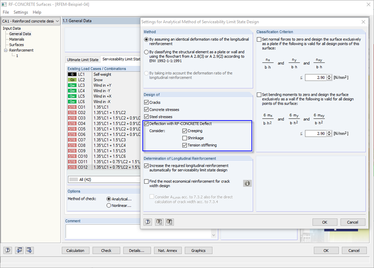
The detection of the crack state can be set in the Serviceability Configuration. The following options are available:

(a) Crack state is calculated based on the corresponding load;
(b) Crack state based on the corresponding characteristic combination (CO) of the SLS design situation;
(c) Crack state determined as an envelope from all SLS design situations;
(d) Crack state independent of the load.

Fig. 1.2: Serviceability Configuration

If you select the Crack state is calculated based on the corresponding load option, the crack state (distribution coefficient ζ_d) is calculated based only on the current load (load combination).

If you select the Crack state based on the corresponding characteristic combination (CO) of the SLS design situation option, the distribution coefficient ζ_d is calculated as the maximum of all corresponding loads. The corresponding loads can be defined in the load combination definition.

Fig. 1.3: Corresponding Loads
If you select the Crack state determined as envelope from all SLS design situations option, the distribution coefficient ζ_d is calculated as the maximum from all design situations. If you select the Crack state independent of load option, the distribution coefficient is always 1.0.

1.6.4. Design Situations

In general, deflection is calculated for quasi-permanent loads. However, it is possible to select desired design situations (in the Serviceability Configuration, option User-defined assignment of design situation type) for which deflection is to be calculated.

The following serviceability design situation types can be selected:

- Quasi-permanent,
- Frequent,
- Characteristic.

A limit value for the deflection can be specified for each type (see Fig. 1.2). In addition, the desired design situations are also specified for concrete design.

Fig. 1.4: Setting of Design Situations for Concrete Design
The setting in concrete design is crucial for the detection of the crack state (especially when selecting whether the detection is based on corresponding loads or on all serviceability design situations).

In other words:
- If a design situation is deactivated in the serviceability configuration, but activated in the concrete design settings, this design situation is taken into account.
- If a design situation is activated in the serviceability configuration, but deactivated in the concrete design settings, this design situation is not taken into account.

1.7. Cross-Section Properties for Deformation Analysis

In the material stiffness matrix D for the deformation analysis, the program requires the cross-section properties in each reinforcement direction, depending on the crack state. These are:

(a) Moment of inertia to the ideal center of gravity I_ф;
(b) Moment of inertia to the geometric center of gravity of the cross-section I_0,c;
(c) Ideal cross-sectional area A_ф;
(d) Eccentricity of the ideal center of gravity e_ф to the geometric center of gravity.

A mean strain ε_ф and a mean curvature κ_ф are calculated by interpolation between the uncracked and cracked states according to EN 1992-1-1, Equation (7.18):

The deformation in the uncracked and cracked state c (states I and II) is calculated according to the following equations:

The ideal cross-section properties are calculated for the ideal center of gravity of the cross-section. The influence of shrinkage is taken into account by the factor k_sh,c,ф:

If the axial force is not equal to zero, the cross-section properties are calculated to the geometric center of gravity of the cross-section, taking into account the eccentricity:

1.8. Material Stiffness Matrix D (Members)

The axial stiffness EA and the bending stiffness EI_y,0 are only calculated in the reinforcement direction ф = 1 (direction of the member) as follows:

1.9. Material Stiffness Matrix D (Surfaces)

When calculating the cross-section properties, the initial value of the Poisson's ratio ν_init is reduced independently in both directions according to the following equation:

The material stiffness matrix is calculated according to the theory for orthotropic surfaces.

1.9.1. Bending Stiffness – Plates and Shells

The bending stiffnesses in the reinforcement directions ф are determined as follows:
For shells:

For plates:
The non-diagonal component of the material stiffness matrix is identical for plates and shells:
For shells, the differences in bending stiffness based on the moments of inertia are compensated by the eccentricity components in the material stiffness matrix.

1.9.2. Torsional Stiffness of Plates and Shells

The elements of the stiffness matrix are calculated for plates and shells as follows:

1.9.3. Shear Stiffness of Plates and Shells

The elements of the stiffness matrix for shear are not reduced in the deformation analysis. They are determined from the shear modulus G of the ideal cross-section and the cross-section depth h. The expression is identical for shells and plates:

1.9.4. Membrane Stiffness of Shells

The membrane stiffnesses in the reinforcement directions φ are calculated as follows:

The non-diagonal part of the material stiffness matrix is determined by:

The component of the shear stiffness is:

1.9.5. Eccentricity – Shells

The elements of the stiffness matrix for the eccentricity of the center of gravity (ideal cross-section) in the reinforcement direction ф are calculated as follows:

The non-diagonal part of the material stiffness matrix is determined by:

The eccentricity component for torsion is calculated as follows:

1.9.6. Test for Positive Definiteness

The positive definiteness of the material stiffness matrix D is tested using a modified SYLVESTER'S criterion (taking into account the zero blocks).

If the stiffness matrix D is not positive definite, the non-diagonal components of the material stiffness matrix are successively set to zero. In extreme cases, only the positive components of the main diagonal remain.

1.10. Calculation of Deflections

The deflections of an object (a member or a surface) are determined using the previously calculated stiffness matrix D. The design value (design ratio) is calculated from the deflection and the limit value.

1.10.1. Corresponding Load

If a corresponding load is assigned to the main load, the final deflection is calculated as the sum of the individual values. The main load combination is calculated without time-dependent properties (creep and shrinkage) and should therefore be short-term (frequent or characteristic). The corresponding load combination, on the other hand, is always calculated with time-dependent properties, and should therefore be long-term (quasi-permanent). If more than one corresponding load is assigned, the one with the highest deflection value is taken into account.

The total deflection is calculated as follows:

1.11. Differences Between RFEM 5 and RFEM 6

Calculation of Depth of Concrete Compression Zone
In RFEM 5, the depth of the concrete compression zone is calculated based on the net cross-section depth, while RFEM 6 uses the gross cross-section depth. This approach ensures a faster and clearer calculation, which also allows for better traceability of the results. This simplification maintains the accuracy of the calculation at a high level, so that the results do not show any significant differences in practice. RFEM 6 thus provides a more efficient solution with consistently precise results.

Distribution Coefficient of Reinforcement
The distribution coefficient, which describes the stress distribution across the cross-section, was determined in RFEM 5 solely on the basis of the long-term stress. This means that only the stress acting over a longer period of time was taken into account. In RFEM 6, the calculation approach has been further developed so that the maximum of both the long-term and short-term stress is now taken into account. This change ensures a more realistic representation of the actual stress conditions in the cross-section.