Applying the finite element method, results are determined for the FE mesh nodes. These nodal values are smoothed by an interpolation method so that you can see a continuous distribution of internal forces, deformations, or stresses in the graphic.
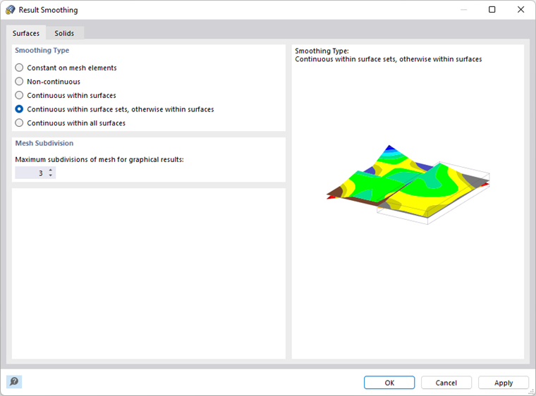
To open the settings for result smoothing, click Result Smoothing in the Calculate menu. In the "Result Smoothing" dialog box, you can adjust the smoothing for surface and solid results.
Surfaces
The Surfaces tab controls whether and how surface results are interpolated.
Smoothing Type
The individual options are illustrated by the following example.
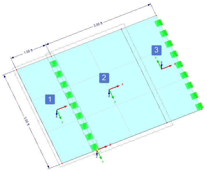
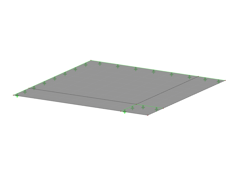
A steel plate with a thickness of 3 cm, including cantilever, is simply supported on two lines. The plate is not modeled by a complete surface, but by three surfaces with the same properties lying side by side. The local z-axes of the surfaces between the supports (Nos. 2 and 3) are directed in opposite directions. The two surfaces in the support area (Nos. 1 and 2) with aligned axes are combined in one surface set.
The steel plate is stressed only by its self-weight. The FE length is 1 m. This element size certainly does not provide precise results; it is only intended to illustrate the result displays of the individual smoothings.
Constant on Mesh Elements
The values of FE nodes are averaged and displayed as constant distributions on each element. This type of result smoothing is recommended for plastic material models.
Non-Continuous
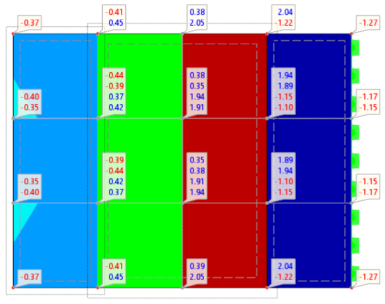
The display shows the values of FE nodes resulting from the displacements and rotations of each single element. Therefore, several values are displayed for each FE node.
For the graphical display, a surface is placed through the corner values of each element. Since the results of the adjacent elements are not taken into account, there is a discontinuous distribution (see cantilevered surface).
Continuous Within Surfaces
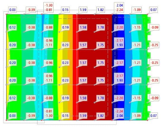
The results in grid points show how the values of FE nodes are interpolated. The averaging ends at the surface boundary. This may lead to discontinuities between adjacent surfaces; for example, along the support area of the cantilevered surface. However, the separation is correct for the results between the supports because the moments of the two surfaces have different algebraic signs.
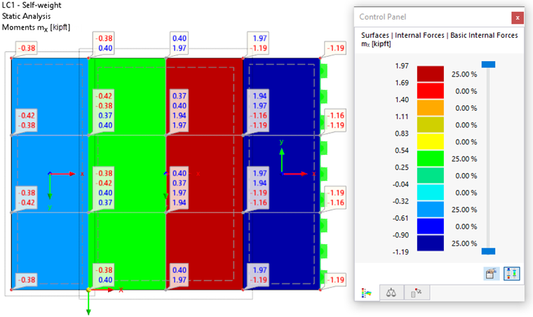
Continuous Within Surface Sets, Otherwise Within Surfaces
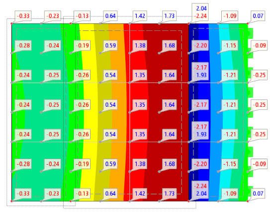
The values of the FE nodes are averaged separately for each surface. If there are surface sets, the interpolation also takes into account the adjacent areas of the surfaces included in the surface set. Thus, as shown in the example, the continuous effect of the surfaces in the support area is determined.
This smoothing option is preset because it provides the best results in most cases.
Continuous Within All Surfaces
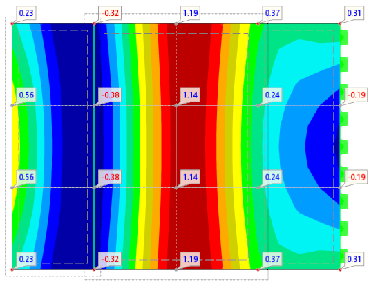
This display mode averages the values beyond the surface boundaries. It leads to a continuous distribution between adjoining surfaces, which is not correct for our example.
For this display type, each of the following conditions must be fulfilled to prevent incorrect result diagrams from being displayed:
- The axis systems of the surfaces are aligned in the same direction.
- At most, two surfaces are adjacent to each other.
- The surfaces lie in one plane.
- The boundary line has no line hinge.
Mesh Subdivision
The "Maximum subdivisions of mesh" describe the accuracy with which the graphical distributions in the finite elements are determined.
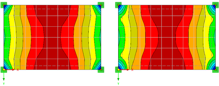
The following example contrasts the distributions of the surface moments mx having "0" and "3" divisions.
Solids
The Solids tab controls whether and how the results available on the boundary surfaces of the solid are interpolated.
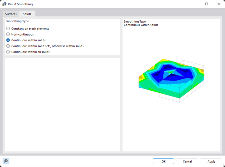
The functions of the options available in the "Smoothing Type" dialog section correspond to those described for surfaces.