1379x

000483

2024-01-16

Select Manual

Overview

Graphical User Interface and Settings

Load Cases and Combinations

Results by Solid

You can display the results for solids graphically using the Solids navigator category. You find the numerical results of solids in the Results by Solid table category.

01 Results by Solid in Table

Info

Both the table and graphic show the results available on the boundary surfaces of the solid. To check the results inside the solid, activate the On FE mesh points option in the Values on Surfaces category in the lower navigator section. Then, you can read off the values within the solid using a clipping plane (see Clipping Planes chapter).

Deformations

The Results by Solid in Table image shows the table with deformations of the boundary surfaces. Displacements and rotations are displayed in the surface grid points (see Surfaces chapter).

Tip

For small surfaces, the grid's standard mesh size of 0.5 m may cause only a few grid points to exist. In this case, adjust the number or distance of grid points to the surface size.

The deformations have the following meaning:

\|u\|	Absolute value of total displacement
u_X	Displacement in direction of global axis X
u_Y	Displacement in direction of global axis Y
u_Z	Displacement in direction of global axis Z
φ_X	Rotation about global axis X
φ_Y	Rotation about global axis Y
φ_Z	Rotation about global axis Z

Stresses

02 Selecting Solid Stresses in Navigator

03 Stresses of Solids in Table

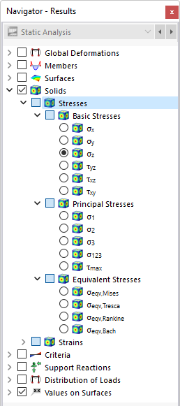
In the navigator, define the stresses to be displayed on the boundary surfaces of solids. The table lists the stresses of these surfaces according to the specifications set in the Result Table Manager .

The solid stresses are divided into the following categories:

Basic Stresses
Principal Stresses
Equivalent Stresses

Unlike surface stresses, solid stresses cannot be described by simple equations. The basic stresses σ_x, σ_y, and σ_z including the shear stresses τ_yz, τ_xz, and τ_xy are determined directly by the computation kernel.

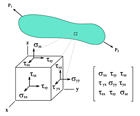
If a cube with the edge lengths d_x, d_y, and d_z is cut out of a multiaxial stressed object, the stresses available in each cube surface can be decomposed into normal and shear stresses. If neither the spatial force nor stress differences on parallel surfaces are considered, the stress condition in the cube's local coordinate system can be described by nine stress components.

04 Solid Element with Stress Components

The matrix of the stress tensor is the following:

S = [\begin{matrix} σ_{x} & τ_{xy} & τ_{xz} \\ τ_{yx} & σ_{y} & τ_{yz} \\ τ_{zx} & τ_{zy} & σ_{z} \end{matrix}]

Matrix of Stress Tensor

The principal stresses σ₁, σ₂, and σ₃ result from the eigenvalues of the tensor as follows:

\det (S - σ E) = 0

E	3x3 unit matrix

Principal Stresses

The maximum shear stress τ_max is determined according to Mohr's circle:

τ_{\max} = \frac{1}{2} (σ_{1} - σ_{3})

Maximum Shear Stress

Tip

The σ₁₂₃ navigator entry allows you to graphically display the trajectories of the principal stresses.

The equivalent stresses σ_eqv according to von Mises can be determined by two equivalent formulas.

σ_{v, Mises} = \sqrt{\frac{1}{2} [(σ_{1} - σ_{2})^{2} + (σ_{1} - σ_{3})^{2} + (σ_{2} - σ_{3})^{2}]}

Equivalent Stress σ_v,Mises from Principal Stresses

σ_{v, Mises} = \sqrt{σ_{x}^{2} + σ_{y}^{2} + σ_{z}^{2} - σ_{x} σ_{y} - σ_{x} σ_{z} - σ_{y} σ_{z} + 3 (τ_{x y}^{2} + τ_{x z}^{2} + τ_{y z}^{2})}

Equivalent Stress σ_v,Mises from Basic Stresses

To determine the equivalent stress σ_eqv according to Tresca , the differences from the principal stresses are examined in order to determine the maximum value.

σ_{v, Tresca} = max (|σ_{1} - σ_{2}|; |σ_{2} - σ_{3}|; |σ_{3} - σ_{1}|)

Equivalent Stress σ_v,Tresca

The equivalent stress σ_eqv according to Rankine is determined from the greatest absolute values of the principal stresses.

σ_{v, Rankine} = max (|σ_{1}|; |σ_{2}|; |σ_{3}|)

Equivalent Stress σ_v,Rankine

To determine the equivalent stress σ_eqv according to Bach , the principal stress differences are examined, taking into account the Poisson's ratio ν, in order to determine the maximum value.

σ_{v, Bach} = max [|σ_{1} - ν (σ_{2} + σ_{3})|; |σ_{2} - ν (σ_{3} + σ_{1})|; |σ_{3} - ν (σ_{1} + σ_{2})|]

Equivalent Stress σ_{v, Bach}

Strains

05 Selecting Solid Strains in Navigator

06 Strains on Solids in Table

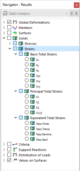
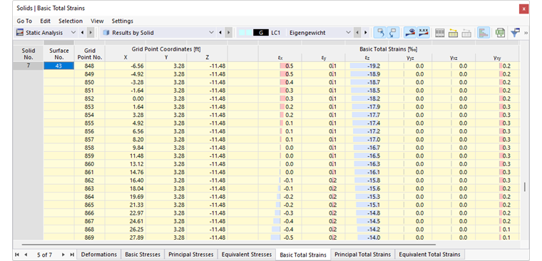
In the navigator, define the strains to be displayed on the boundary surfaces of solids. The table lists the strains of these surfaces according to the specifications set in the Result Table Manager .

The solid strains are divided into the following categories:

Basic Total Strains
Principal Total Strains
Equivalent Total Strains

The basic total strains including shear strains are determined directly by the computation kernel. The general definition of the tensor for the spatial strain state is as follows:

ε = [\begin{matrix} ε_{x x} & ε_{x y} & ε_{x z} \\ ε_{y x} & ε_{y y} & ε_{y z} \\ ε_{z x} & ε_{z y} & ε_{z z} \end{matrix}]

Tensor for Strain State

The elements of the tensor are defined as follows:

ε_{i j} = \frac{1}{2} (\frac{\partial u_{i}}{\partial x_{j}} + \frac{\partial u_{j}}{\partial x_{i}})

Tensor Elements

The principal total strains ε₁, ε₂, and ε₃ are determined from the basic strains.

Tip

The ε₁₂₃ navigator entry allows you to graphically display the trajectories of the principal strains.

The equivalent total strains ε_eqv are determined according to four different stress hypotheses as follows.

ε_{v, Mises} = \frac{1}{1 + ν} \sqrt{{ε_{x}}^{2} + {ε_{y}}^{2} + {ε_{z}}^{2} - ε_{x} ε_{y} - ε_{y} ε_{z} - ε_{z} ε_{x} + \frac{3}{4} ({γ_{x y}}^{2} + {γ_{y z}}^{2} + {γ_{x z}}^{2})}

Comparative Total Strain ε_v,Mises

ε_{v, Tresca} = \max (|R_{1} - R_{2}|; |R_{2} - R_{3}|; |R_{3} - R_{1}|)

R	Matrix (see below)

Comparative Total Strain ε_v,Tresca (Maximum of Eigenvalue Differences According to Matrix R)

ε_{v, Rankine} = \max (|R_{1}|; |R_{2}|; |R_{3}|)

R	Matrix (see below)

Comparative Total Strain ε_v,Rankine (Maximum of Eigenvalues According to Matrix R)

ε_{v, Bach} = \max (|R_{1} - ν (R_{2} + R_{3})|; |R_{2} - ν (R_{3} + R_{1})|; |R_{3} - ν (R_{1} + R_{2})|)

R	Matrix (see below)

Comparative Total Strain ε_v,Bach (Maximum of Eigenvalue Differences According to Matrix R Taking into Account Poisson's Ratio ν)

R = \frac{1}{1 + ν} [\begin{matrix} \frac{(1 - ν) ε_{x} + ν (ε_{y} + ε_{z})}{1 - 2 ν} & \frac{γ_{x y}}{2} & \frac{γ_{x z}}{2} \\ \frac{γ_{x y}}{2} & \frac{(1 - ν) ε_{y} + ν (ε_{x} + ε_{z})}{1 - 2 ν} & \frac{γ_{y z}}{2} \\ \frac{γ_{x z}}{2} & \frac{γ_{y z}}{2} & \frac{(1 - ν) ε_{z} + ν (ε_{x} + ε_{z})}{1 - 2 ν} \end{matrix}]

Matrix R

Parent section

Results