


A static analysis setting (SA) specifies the rules according to which load cases and load combinations are calculated. Three standard analysis types are preset.
Main
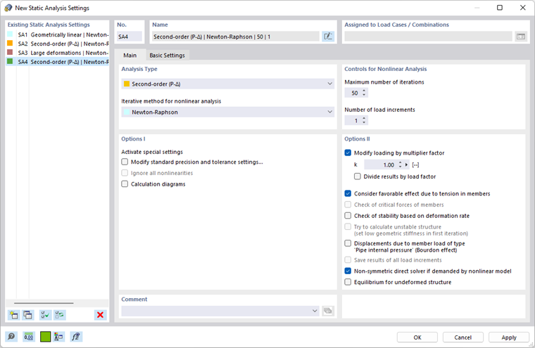
The Main tab manages the settings for the structural analysis and elementary calculation parameters.
Analysis Type
This dialog section controls the calculation theory according to which load cases and load combinations are analyzed. In the "Analysis Type" list, three approaches are available for selection.
Geometrically linear
When calculating according to the geometrically linear analysis (first-order), the equilibrium is analyzed on an undeformed structural system. A linear analysis is carried out because deformations of the components are not included in the calculation.
Load cases are calculated according to the geometrically linear analysis by default.
Second-order (P-Δ)
In the "structural" second-order analysis, the equilibrium is determined on a deformed structural system. Deformations are assumed to be small. Axial forces in the system have an impact on an increase in bending moments. Thus, this analysis comes into effect when axial forces are significantly greater than shear forces.
Load combinations are calculated nonlinearly by default according to the second-order analysis.
Large deformations
The large deformation analysis (third-order or theory of large deformations) considers longitudinal and transversal forces in the calculation. After each iteration step, the stiffness matrix of a deformed system is created. Loads are handled in a differentiated manner: A load defined in the global direction keeps its direction if finite elements are twisted. If the load acts in the direction of a local member or surface axis, it changes its direction according to the element's twisting.
If the model includes cable members or membrane surfaces, the calculation according to the large deformation analysis is preset.
Iterative Method for Nonlinear Analysis
Depending on the analysis type, various methods are available to solve the nonlinear algebraic system of equations.
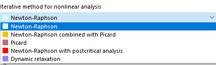
Newton-Raphson
The approach according to Newton-Raphson is preset for the large deformation analysis. The nonlinear equation system is solved numerically by means of iterative approximations with tangents. The tangential stiffness matrix is determined as a function of the current deformation state; it is inverted in each iteration cycle. In the majority of cases, a fast (quadratic) convergence is reached.
Newton-Raphson Combined with Picard
The approach according to Picard is applied first. After a few iterations, a switch is made to the Newton-Raphson method. The basic idea of this approach is to use the relatively "insensitive" Picard method for the first iteration steps in order to avoid instability messages. This initial approximation is followed by the fast method according to Newton-Raphson to find the ultimate state of equilibrium.
Picard
The method according to Picard, also known as the secant method, can be understood as a finite-difference approximation of the Newton-Raphson method. The difference between the current and the original iteration run in the current load increment step is considered. This method usually converges slower than the calculation method according to Newton-Raphson. However, it also proves to be less sensitive to nonlinear problems, which makes the calculation more stable.
Newton-Raphson with postcritical analysis
This method is suitable for solving post-critical analyses where an area with instability has to be overcome. If an instability is available and the stiffness matrix cannot be inverted, the stiffness matrix of the last stable iteration step is used. This matrix is used for further calculations until the stability range is reached again.
Dynamic relaxation
The final method is suitable for calculations according to the large deformation analysis and for solving problems regarding the post-critical issues. In this approach, an artificial time parameter is introduced. Taking into account inertia and damping, the failure can be handled as a dynamic problem. This approach uses the explicit time-integration method; the stiffness matrix is not inverted. No part of the model is allowed to have a specific weight of zero when calculating with dynamic relaxation.
This method also includes the Rayleigh damping, which can be defined via the constants α and β according to the following equation with the derivatives with respect to time:
|
M |
Concentrated (diagonal) mass matrix |
|
C |
Diagonal damping matrix C = αM + βdiag[K11(u),K22(u),...,Knn(u)] |
|
K |
Stiffness matrix |
|
f |
Vector of external forces |
|
u |
Discretized displacement vector |
Controls for Nonlinear Analysis
The "Maximum number of iterations" defines the highest number of calculation runs for an analysis according to the second-order or large deformation analysis, as well as for non-linearly acting objects. When the calculation reaches the limit without reaching an equilibrium, a corresponding message appears. Then, you can decide if you want to display the results.
The "Number of load increments" is relevant for calculations according to the second-order or large deformation analysis. When considering large deformations, it is often difficult to find an equilibrium. Instabilities can be avoided by applying loading in several steps. For example, if you specify two load increments, half of the load is applied in the first step. It is iterated until the equilibrium is found. In the second step, the full loading is then applied to the already deformed system and iterated again until equilibrium is reached.
Options I
In this dialog section, you can activate various "special settings" to manipulate calculations according to the second-order or large deformation analysis.
Modify standard precision and tolerance settings
When you select the "Modify standard precision and tolerance settings" check box, the Precision and Tolerance tab is added to the dialog box. There, you can adjust the convergence criteria.
Ignore all nonlinearities
With the "Ignore all nonlinearities" check box, you can deactivate the nonlinear properties of elements for the calculation. Tension members, for example, remain in the model whenever compressive forces occur. However, you should suppress the non-linear properties only for test purposes; for example, to find the cause of an instability. Incorrectly defined failure criteria are sometimes responsible for calculation break-offs.
Options II
Modify loading by multiplication factor
After ticking the check box, you can define a factor k by which all loads are to be multiplied.
Older standards claim to multiply loads globally by a certain factor in order to increase effects according to the second-order analysis for stability designs. In turn, the design must be carried out with the service loads. Both requirements can be met by entering a factor greater than 1 and activating the "Divide results by load factor" check box.
For analyses according to current standards, the loading should not be edited by means of factors. Instead, the partial safety and combination factors are to be taken into account for the superposition in the design situations.
Consider favorable effect due to tension in members
Tensile forces have a favorable effect on pre-deformed structural systems. Thus, the deformation is reduced and the structure is stabilized. Usually, we benefit from this effect in calculations according to the second-order and large deformation analysis; for example, for halls with bracings or general structures subjected to bending. Relief due to tension force effects for beams trussed from below (beams with supporting ties or cables) may result in an unwanted reduction of deformations and internal forces.
Check of stability based on deformation rate
If you tick the check box, RFEM checks how the deformations develop during the calculation. If the displacements or torsions increase strongly and exceed a limit in the program, the calculation stops and a message about instability is displayed.
Try to calculate an unstable structure
With this check box, you can try to make an unstable model calculable: In the first calculation step, RFEM applies small springs stabilizing the model for the first iteration. Once a stable initial state is reached, the springs are removed for subsequent iterations.
Displacements due to member load of "Pipe internal pressure" type
The check box is relevant for the member load called pipe internal pressure. The Bourdon effect describes the effort of a bent pipe to straighten under the influence of pressure. Both perimeter stresses and axial stresses caused by internal pressure load lead to longitudinal strain of the pipe, considering material stiffness and transversal strain.
See this Technical Article describing an example of how the internal pressure of pipes is calculated.
Save results of all load increments
If the loading is applied incrementally (see Controls for Nonlinear Analysis), you can use this check box to force the output of intermediate results in order to check the results of the individual load increments.
Non-symmetric direct solver
For a nonlinear material model (see the chapter Nonlinear Material Behavior) with non-symmetrical properties for tension and compression, a non-symmetrical direct equation solver is used. The check box also allows you to use this equation solver for other material models, such as the Isotropic Nonlinear Elastic material model.
Equilibrium for undeformed structure
The check box allows you to analyze a non-deforming structure; that is, a structural system whose deformations remain zero. This analysis option may be useful when, for example, a system is subjected to stress due to a load case, while the resulting deformations can be considered to have subsided.
One field of application for calculating the equilibrium for the undeformed structure is the primary stress state of the geotechnical analysis. The acting stresses resulting from the preload of the soil are to be determined in the scope of a load case or combination. However, the deformations of such a load case or combination are not of interest and, therefore, not a subject of further use.
Basic Settings
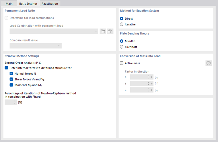
The Basic Settings tab manages the basic specifications for the calculation.
Permanent Load Ratio
The "Determine for load combinations" check box offers the possibility to determine the ratio of a permanently acting load in a load combination. Select the load combination in the list, or create a new load combination with the
 button. Then, in the "Compare result value" list, you can define the ratios that have a static or variable effect.
The ratio of the permanent load can be considered as conforming to the standards in the design.
Method for Equation System
Both options control the methods used for solving the equation system. To prevent misunderstandings: Even when the equation system is solved directly, an iterative calculation is carried out if there are non-linearities or if calculations are performed according to the second-order or large deformation analysis. "Direct" and "Iterative" refer to the data management during the calculation.
Which solver method yields faster results depends on the complexity of the model as well as on the size of the available main memory (RAM). For small and medium-sized systems, the direct method is more efficient.
For very large and complex systems, the iterative method leads to results more quickly.
Plate Bending Theory
Surfaces can be calculated according to the "Mindlin" or "Kirchhoff" bending theories. In the calculation according to Mindlin, shear force deformations are included; according to Kirchhoff, they are not taken into account. The Mindlin calculation option is, therefore, suitable for relatively thick plates and shells used in solid construction, while the Kirchhoff option is recommended for surfaces that are relatively thin, such as metal sheets in steel construction.
Iterative Method Settings
The check boxes in this dialog section are important for the "Second-order (P-Δ)" analysis.
Refer internal forces to deformed structure
The internal forces of members are usually output in relation to the modified position of the member coordinate systems that is present in the deformed system. If you want the output to refer to the undeformed initial system, you can define the relevant member internal forces and moments by deactivating the corresponding check boxes.
Percentage of iterations of Newton-Raphson method in combination with Picard
The method according to Picard is based on secant stiffenings, while the Newton-Raphson method is based on tangent stiffenings. With the calculation option Newton-Raphson combined with Picard, secant stiffnesses are used in the first iterations before tangent stiffnesses are applied for the remaining iterations. The ratio of the first iterations with secant stiffnesses is related to the total number of iterations.
Conversion of Mass into Load
Loads can be defined not only as forces and moments, but also in the form of masses. However, masses have no effect in the structural analysis. If you want to consider them, select the "Active mass" check box. Then, enter the "Factor in direction" to describe the effect of the mass. Thus, the masses are converted into forces before the calculation starts, and they are included in the determination of internal forces and moments.
Use the
 button to switch between entering the mass factor and entering the acceleration directly. The name of the input fields is adjusted accordingly.
Reactivation
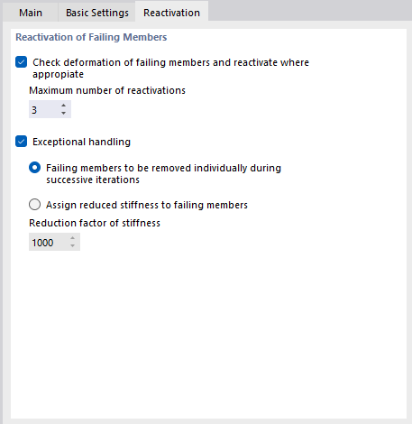
The Reactivation tab is available as soon as a member with non-linear properties exists in the model. In this tab, you can control how failing members are treated in the analysis.
Failing members are often the cause of instability problems; for example, when a member model is stiffened by tension members. Because of frame column contractions due to the vertical load, the tension members receive small compressive forces in the first calculation step. They are removed from the system. In the second step, the model becomes unstable without these tension members. With the options in the "Reactivation of Failing Members" dialog section, you can try to achieve a calculation without an error message.
Check deformation of failing members and reactivate where appropriate
RFEM analyzes nodal displacements in each iteration. For example, if the member ends of a failed tension member move away from each other, the member is used again in the stiffness matrix.
Reactivating members may be problematic in some cases: A member is removed after the first iteration, reintroduced after the second iteration, removed again after the third, and so on. The calculation would run through this loop until the maximum possible number of iterations are reached without converging. The "Maximum number of reactivations" prevents this effect. You can define how often a member element may be reinserted before it is finally removed from the stiffness matrix.
Exceptional handling
If you tick the "Exceptional handling" check box, you can select from two methods for dealing with failing members. They can be combined with the reactivation described above.
- Failing members to be removed individually during successive iterations
After the first iteration, RFEM does not, for example, remove all tension members with a compression force at once, but only the tension member with the greatest compressive force. In the second iteration, only one member is then missing in the stiffness matrix. Subsequently, the tension member with the greatest compressive force is removed again. This way, the system often shows better convergence behavior due to redistribution effects.
This calculation option requires more time because the program must go through a larger number of iterations. In addition, it must be ensured that a sufficient Maximum Number of Iterations is provided in the "Main" tab.
- Assign reduced stiffness to failing members
The failed members are not removed from the stiffness matrix, but are instead assigned a very small stiffness. You can define it in the "Reduction factor of stiffness" field: A factor of 1,000 means that the member stiffness is reduced to 1/1,000.
Precision and Tolerance
The Precision and Tolerance tab allows you to influence the convergence and tolerance parameters of the calculation. However, you should change the default settings only in exceptional cases.
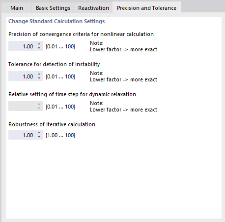
Precision of convergence criteria of nonlinear calculation
If nonlinear effects are acting, or if the second-order or large deformation analysis is performed, the calculation can be influenced by means of convergence criteria.
The change of axial forces in the last two iterations is compared member by member. As soon as this change reaches a specific fractional amount of the maximum axial force, the calculation stops. However, during the iterations it may happen that the axial forces oscillate between two values. You can prevent this pendulum effect by adjusting the "sensitivity".
The precision also affects the convergence criterion for deformation changes in calculations performed according to the large deformation analysis, where geometric non-linearities are considered. The default value is 1.00. The minimum factor is 0.01, the maximum value 100.00. The smaller the value is, the closer the convergence term must be to the comparison term. The result accuracy is increased accordingly.
Tolerance for detection of instability
There are different approaches to analyze the stability behavior of a model. However, none of them is able to detect singular stiffness matrices with absolute reliability.
RFEM uses two procedures to determine the instability: First, the elements on the main diagonal of the stiffness matrix are always compared in absolute terms with the same number in the iterations. Second, each element of the main diagonal is analyzed relative to the adjacent number. The tolerance can be adjusted in the field. The smaller the tolerance value is, the closer the model's instability limit is moved to the exact instability location. The result accuracy is increased accordingly.
Relative setting of time step for dynamic relaxation
The time parameter controls the calculation as per the method of dynamic relaxation. The smaller the value, the smaller the time step by which all response fluctuations are recorded. The accuracy of the results is increased accordingly.
Robustness of iterative calculation
In the case of convergence problems with the Newton-Raphson method, the robustness can be strengthened in order to prevent the solution from "skipping". Reducing the value reduces the number of possible solutions in the presence of a non-converging horizontal solution branch, and thus also reduces the possibility of a valid result within the specified iterations. It may be necessary to increase the maximum number of iterations.