Surfaces

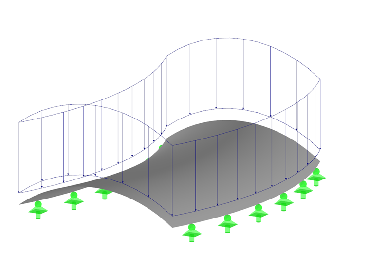
Surfaces describe the geometry of plane or curved structural components whose surface dimensions are considerably larger than their thicknesses. The stiffness of a surface results from its material and thickness. When generating the FE mesh, 2D elements are created on surfaces. These are applied for the calculation in the surface's centroidal axis.

To enter a surface, you can use existing boundary lines. If you describe the surface graphically using the options in the Navigator shortcut menu or the toolbar buttons (see image Buttons for Plane Surfaces), the definition lines are automatically created after defining the surface parameters and clicking OK in the dialog.

The Basic tab manages elementary surface parameters. By checking check boxes, further tabs are added in which you can make the specific specifications.

Stiffness type

The stiffness type controls the way in which internal forces can be absorbed or which properties are assumed for the surface. Various types are available for selection in the list.

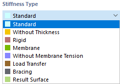
Standard

The surface transfers moments and membrane forces. This approach describes the general behavior of a homogeneous and isotropic surface model. The stiffness properties of the surface are direction-independent.

Without thickness

The surface has no stiffness. This type is to be used for the boundary surfaces of a solid.

Rigid

This stiffness type can be used to model very stiff surfaces in order to model a rigid connection between objects.

Membrane

The surface has a uniform stiffness in all directions. However, only membrane forces in tension (n_x, n_y) and membrane shear forces (n_xy) are transferred. In the case of compressive and shear forces as well as moments, the affected surface elements fail.

Without membrane tension

Only moments and membrane forces in compression are transferred. If membrane forces cause tension, the affected surface elements fail (example: hole bearing).

Load transfer

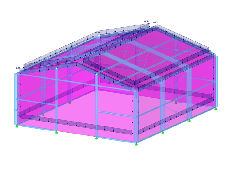
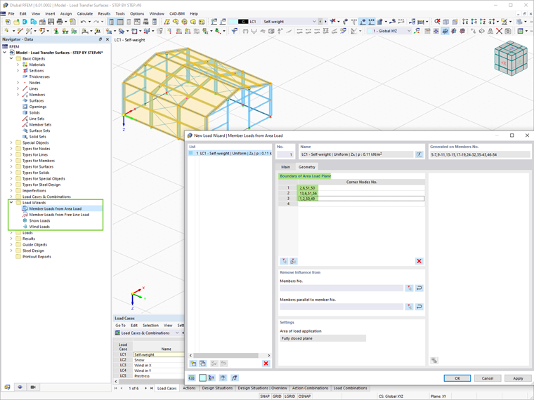
This type allows surface loads to be applied to areas that are not filled with surfaces, such as wind loads on windows or the members of a hall. The load of this surface is distributed to the edges or the integrated objects. If member loads are generated, the load is converted to the true member lengths in the global directions (load directions X_L, Y_L, Z_L). The surface itself has no stiffness.

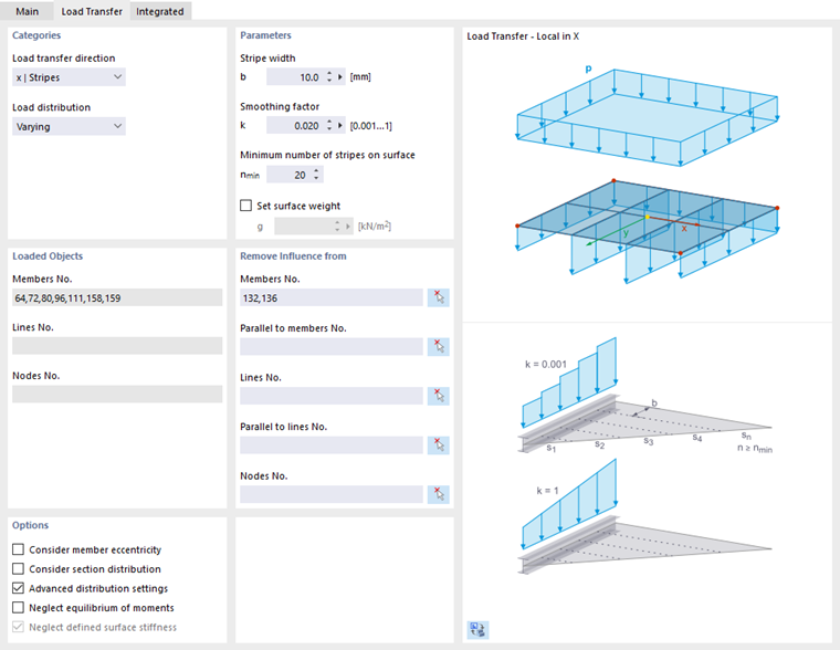
You can define the criteria for the load transfer in the Load transfer tab.

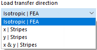
The 'load transfer direction' describes the direction(s) in which the load is to be applied to the objects. The list offers selection options for an isotropic distribution based on an FEM analysis as well as for an orthotropic arrangement on surface strips that are used to determine the load intake width in one or both local surface axes.

With the 'Isotropic | FEM' option, RFEM uses a separate partial model to determine the load distribution, in which the surface is represented by a rigid surface element. All objects integrated into the surface (members, line and nodal supports, lines connected with model elements, couplings or nodes, etc.) are replaced by rigid lines or rigid nodal supports. The reactions of this partial model are then applied as loads for the 3D calculation by RFEM. If certain objects are not to transfer loads, you can specify them in the 'Without effect on' section.

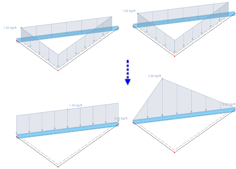
For the load transfer via surface strips, you can define how RFEM should perform the 'load distribution'. By default, the load is distributed to the adjacent objects with a variable distribution. However, if you want to achieve a constant load distribution, select the corresponding entry in the list. The difference between the two variants is contrasted in the following image.

The input options for the 'surface strip width', the 'smoothing factor', and the 'minimum number of strips on the surface' are accessible if the Advanced distribution settings check box is activated in the 'Options' section. Adjustments are only necessary for problematic load distributions. The effect of these parameters is explained in the technical article Advanced Distribution Settings for Load Transfer Surfaces using an example.

For the load transfer surface, you can also define a 'basis weight', for example to take into account the self-weight of a glazing.

In the 'Without effect on' section, you can exclude members, lines, and nodes from the load transfer (for example, bracings). Define the objects individually or select a pattern object that lies parallel to the load-free members or lines.

When the boundary lines of the surface are defined, the loaded members, lines, and nodes are specified in the 'Loaded objects' section. If you want a specific load distribution, check the Load distribution factor check box in the 'Basic' tab. You can then individually define the factors for the load-bearing objects in the Load Distribution Factors tab.

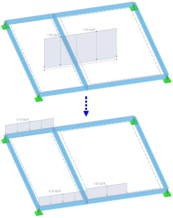
For the load transfer via surface strips, you can take into account the 'member eccentricity' or the 'section distribution' in order to correctly record the geometric position of a member or its distribution (see chapter Cross-section). The 'Neglect rotational equilibrium' check box is not activated by default. This means that the moment from the surface loads is formed at the centroid and balanced with the moment from the member loads at the centroid. For nodal loads, however, this option is irrelevant. The following image shows how a free line load is distributed to the opposite members with and without taking the rotational equilibrium into account.

Stiffening

This stiffness type allows stabilizing effects of trapezoidal sheeting, purlins, and bracings to be taken into account easily and realistically in the modeling.

A stiffening surface is not taken into account as a stiffness-effective object. Rather, it represents the geometric basis for defining the members and objects lying in the stiffening surface and for determining their stiffening effect. Therefore, for a stiffening surface, the Deactivate for Calculation check box is automatically checked and cannot be deactivated.

You can define the criteria of the stiffening surface in the Stiffening, Parameters, and Tolerances tabs.

Stiffening

Two stiffening types are available for selection, which differ fundamentally.

• Surface

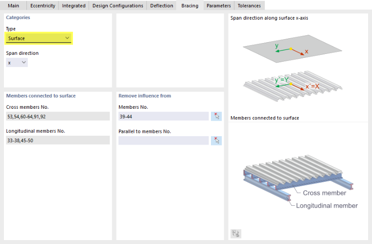
The stiffening effect of a trapezoidal sheeting is represented by an orthotropic surface that is connected to the connected members via rigid couplings. The stiffness of the fasteners is taken into account by line hinges in the rigid couplings.

The 'stress direction' defines the orientation of the trapezoidal sheeting. It influences the orientation of the orthotropic surface and is taken into account when defining the orthotropy properties. The x and y axes refer to the local xyz axis system of the surface.

In the 'Members connected to surface' section, the members that are taken into account as secondary beams and longitudinal beams of the trapezoidal sheeting are automatically entered. These are all members within the defined tolerances in the plane of the stiffening surface and perpendicular or parallel to the stress direction of the trapezoidal sheeting.

The 'Without effect on' section offers the possibility to exclude certain members from the automatic assignment as connected members.

• Member support

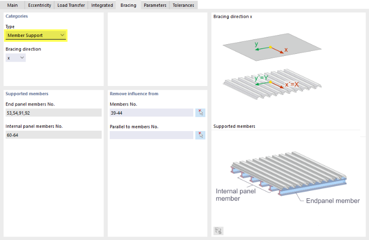
The stiffening effect of trapezoidal sheeting, purlins, or bracings is recorded by member supports on the members of the surface: For these connected members, corresponding member shear panels and rotational restraints are created.

The 'stiffening direction' defines the orientation of the trapezoidal sheeting or the purlins. The x and y axes refer to the local xyz axis system of the surface.

In the 'Supported members' section, the members that limit the end field of the stiffening surface, lie closest to a boundary of the stiffening surface, or are located in an interior field of the surface are automatically entered. The tolerances apply in the plane of the stiffening surface and for the orientation perpendicular to the stiffening direction.

The 'Without effect on' section offers the possibility to exclude certain members from the automatic assignment as connected members.

Parameters

The 'Parameters' tab is adapted to the stiffening type: For a surface, you define the properties of the trapezoidal sheeting and the fasteners; for a member support, you define the stabilizing components.

• Surface

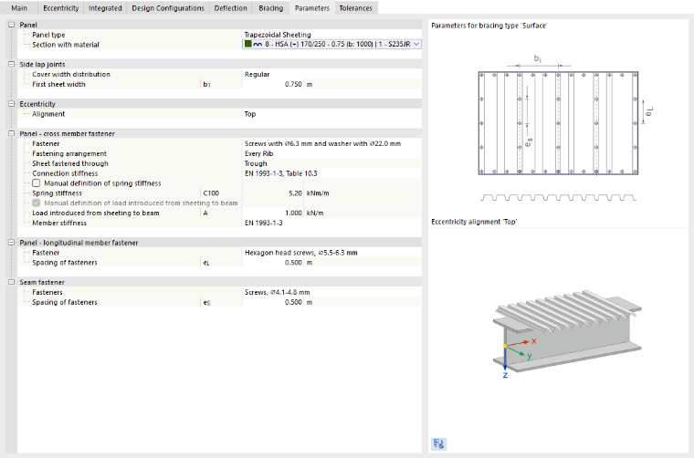
In the 'Panel' category, define the trapezoidal sheeting. In the list, you can select an already defined profile or create a trapezoidal sheeting with the 'New cross-section' option. Use the library that is accessible via the button. The properties required for the orthotropic surface are automatically adopted from the cross-section parameters. They are used for a thickness with the thickness type Shape Orthotropy and the orthotropy type 'Trapezoidal sheeting'.

In the 'Longitudinal joints' category, you define whether the trapezoidal sheets are arranged regularly or irregularly. A separate orthotropic surface is created for each area between two adjacent longitudinal joints. These surfaces are coupled at the longitudinal joints via line hinges. The stiffness of the longitudinal joint connection is taken into account via the spring stiffnesses defined in the line hinges, which result from the flexibility of the fasteners selected in the 'Longitudinal joint fastening' category. The positions of the longitudinal joints are automatically derived from the arrangement of the trapezoidal sheets.

The 'eccentricity' describes the position of the trapezoidal sheeting relative to the connected secondary beams. With the 'Top' option, for example, the trapezoidal sheeting is arranged so that its underside lies on the top side of the secondary beams.

In the 'Panel – secondary beam fastening' category, you define the parameters for connecting the orthotropic surface to the secondary beams. It is done via rigid couplings. The line hinge of the rigid couplings represents the stiffness of the connection including the influence of the profile deformation. Selected fasteners are available for fastening the trapezoidal sheeting to the secondary beams.

For a trapezoidal sheeting in negative position, you can define whether the sheet is fastened on the bottom chord or top chord. For trapezoidal sheets in positive position, the fastening is always on the bottom chord.

The connection of the orthotropic surface to the longitudinal beams is also done via rigid couplings with line hinges, which result from the stiffnesses of the fasteners. In the 'Panel – longitudinal beam fastening' category, some fasteners are available for selection.

In the 'Longitudinal joint fastening' category, you specify the fasteners for the longitudinal joints. Here, too, certain types are available in the list.

• Member support

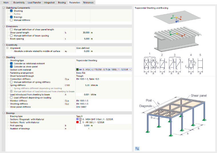
Select which components contribute to stabilization in the calculation. In addition to the 'sheeting', 'purlins', and 'bracings' components, the 'manual stiffness' option is also available. Sheeting and purlins are mutually exclusive. Bracings, however, can be combined with both sheeting and purlins.

In the 'Dimensions' category, define the geometry. The shear panel length is derived by default from the geometry of the stiffening surface but can also be adjusted manually; in both cases, the 'Consider as shear panel' option must be checked in the 'sheeting' category. The crossbeam spacing is also preset automatically as the maximum distance between the members of the end and interior fields. Manual definition is also possible.

The 'eccentricity' describes the position of the trapezoidal sheeting relative to the connected members. With the 'Top' option, for example, the trapezoidal sheeting is arranged so that its underside lies on the top side of the members.

In the 'sheeting' category, you can define the parameters of the trapezoidal sheeting. If you check the 'Consider as rotational restraint' option, the program creates a member support with the Φ_x nonlinearity rotational restraint about x for the members of the end and interior fields. With the 'Consider as shear panel' option, a member support with the nonlinearity shear panel in y or z is generated for each of the members of the end and interior fields. The direction results from the local member axis, which lies in the stiffening surface.

For a sheeting, you can select an already defined profile in the 'Cross-section and material' list or create a trapezoidal sheeting with the 'New cross-section' option. Use the library accessible via the button. Then define the further parameters such as fastening type, determination of the connection stiffness, member and sheet stiffness, etc. If the 'Consider as shear panel' check box is activated, the shear panel stiffness according to DIN 18807 is also taken into account.

For purlin member supports, select the profile of the purlins in the 'Purlins' category and specify the spacing of the purlins. Taking into account further stiffness parameters, member supports with the Φ_x nonlinearity rotational spring stiffness about x are created for the members of the end and interior fields.

In the 'Bracing' category, select the profile of the diagonals and posts. Specify the spacing of the posts and the number of bracings. From these parameters, member supports with the nonlinearity shear panel in y or z are created for the members of the end and interior fields. The direction results from the local member axis, which lies in the stiffening surface.

Tolerances

In the 'Tolerances' tab, you define the permissible deviations according to which members are automatically assigned to the longitudinal and secondary beams (stiffening type Surface) or to the end field and interior field (stiffening type Member support).

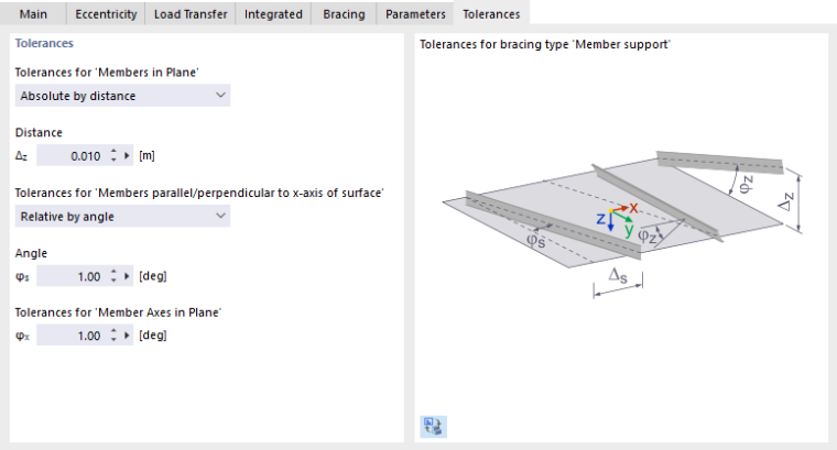
The 'tolerances for members in plane' control the deviation within which members are considered to lie in the stiffening surface. You can define this value absolutely as a distance or relatively by an angle. Analogously, you can define the 'tolerances for members parallel/perpendicular to the x-axis of the surface'.

• Show and hide generated objects of stiffening surfaces

The program generates orthotropic surfaces, rigid couplings, and line hinges from the parameters with the corresponding geometry and stiffness properties. Using the button in the toolbar, you can control whether these generated objects are displayed in the model. Alternatively, use the check box Model → Surfaces → Stiffening in the Navigator – Display.

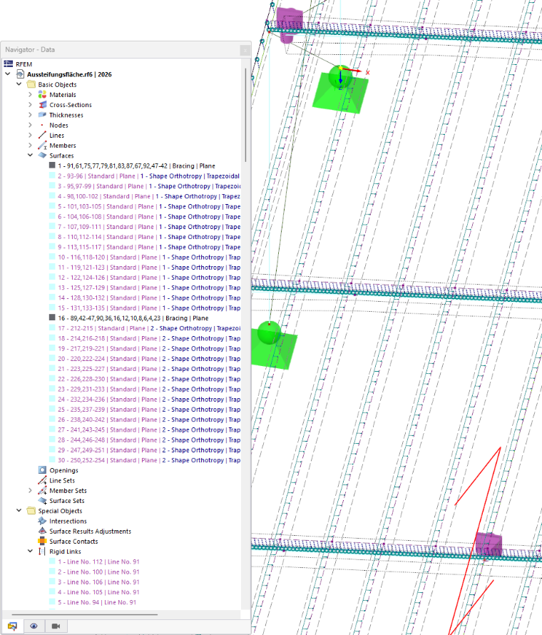
When rendering the full model, the selected trapezoidal sheeting is displayed. This allows you to check the stress direction graphically. The stress direction is also symbolized by a red direction arrow.

• Convert generated objects of stiffening surfaces into standard objects

The generated objects of stiffening surfaces – orthotropic surfaces, rigid couplings, line hinges – are marked in purple in the Navigator – Data and cannot be edited. If you want to edit the objects, the program offers a way to convert them into "real" surfaces. Proceed as follows:

1. Double-click a generated surface or generated line hinge in the Navigator – Data.
2. Click the button at the bottom of the object dialog.

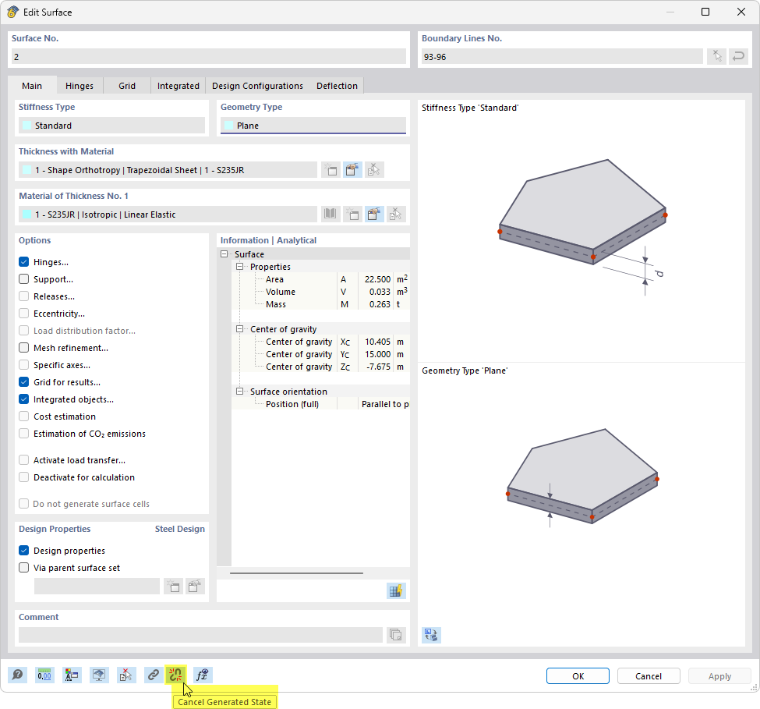
With this function, all generated objects of the stiffening surface are converted into orthotropic standard surfaces and, if necessary, standard hinges. The generated state is thus dissolved and the generated objects are lost as such. Therefore, a corresponding note appears before executing the function.

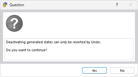
If you have used the function by mistake, you can restore the original state with the undo button . Or you can close the file without saving.

Result surface

This stiffness type makes it possible to convert stresses and forces of other objects into surface internal forces via an integration method. For example, for a solid, you can determine the membrane and bending stresses that are to be designed with different partial safety factors.

You can define further criteria for integrating results in the Result surface tab.

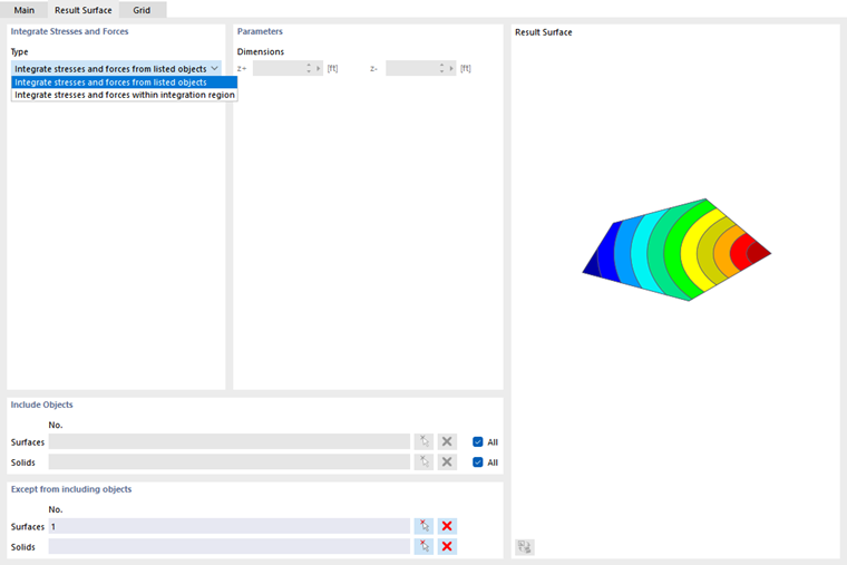
In the 'Integrate stresses and forces' section, select whether the results should be recorded purely object-related or also geometrically within an area. In the 'Include objects' section, define the relevant surfaces and solids. Alternatively, select 'all' objects and then exclude certain elements in the 'Excluded from inclusive objects' section.

If the results of a certain area "below" and "above" the surface are to be integrated, you can define the relevant distances in the 'Parameters' section. They refer to the local z axis perpendicular to the surface plane.

Geometry type

The geometry type describes the formal concept of a surface. Various types are available for selection in the list.

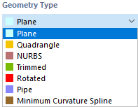
Plane

In a plane surface, all boundary lines lie in one plane. Various shapes of plane surfaces are accessible via the list button.

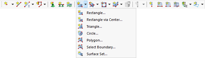
You can define the surface graphically (after clicking OK in the dialog) by dragging a rectangle, circle, etc. If you 'select the boundary', RFEM automatically detects the surface as soon as a sufficient number of boundary lines is defined.

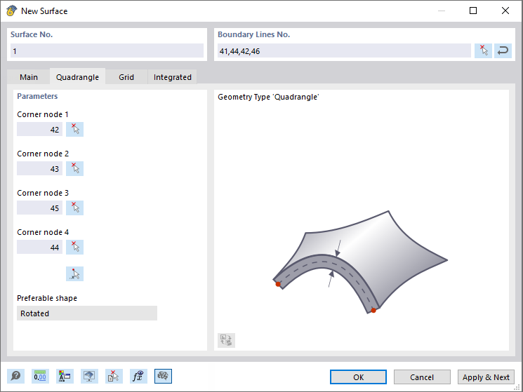
Quadrangle

This surface type describes, in its basic form, a general four-sided surface. Straight lines, arcs, polylines, and splines are possible as boundary lines. This allows curved surfaces to be modeled.

Define the boundary lines of the quadrangle surface in the 'New Surface' dialog. If the closed surface cannot be formed by four lines, more than four lines are also permissible. The four corner nodes are then specified in the 'Quadrangle' tab. They control how the curved surface is spanned.

NURBS

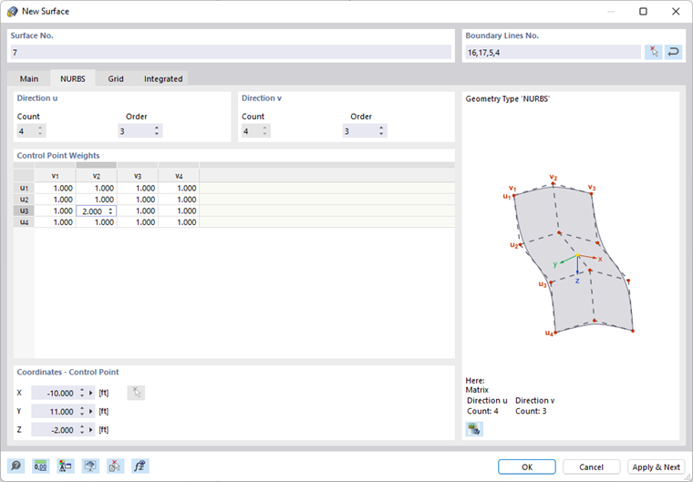
NURBS surfaces are formed from four closed NURBS lines (see chapter Lines). This allows almost any free-form surfaces to be modeled.

Define the boundary lines of the NURBS surface in the 'New Surface' dialog. The respective opposite pairs of NURBS lines must have the same number of control points so that the order of these NURBS lines is "compatible". In the 'NURBS' tab, you can then influence the shape of the surface via the 'control point weights'. The coordinates of the selected control point are given in the 'Coordinates – Control point' section.

Trimmed

If surfaces intersect, you can quickly create the intersection: Select the surfaces and then open the shortcut menu. Various options are available for selection.

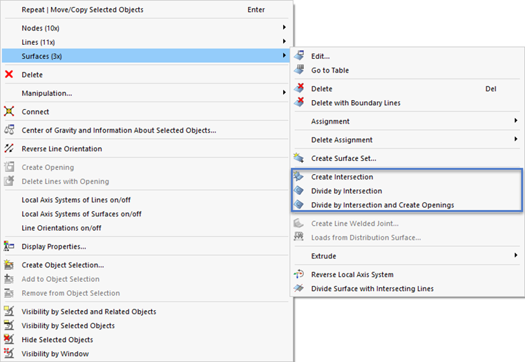
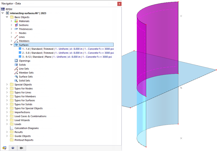
With the 'Create intersection' option, only the intersection line is generated. If you select one of the 'Split by intersection' options, RFEM creates partial surfaces and assigns them the type 'Trimmed'. You can then delete components if, for example, you want to remove protruding surfaces.

Rotation

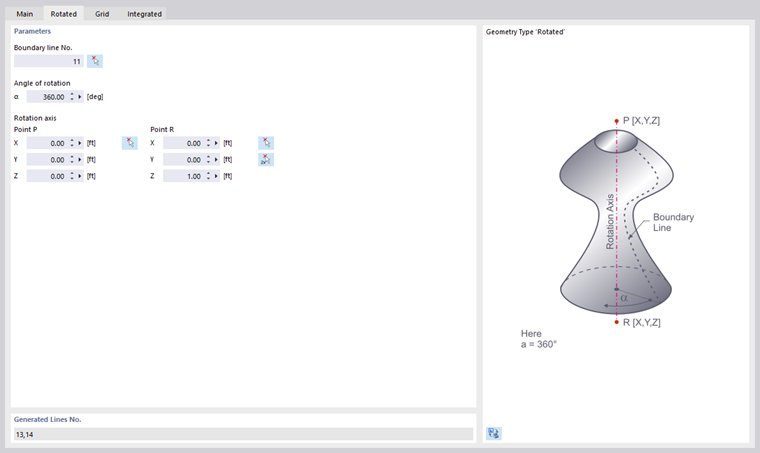
A rotated surface is created when an existing line is rotated about an axis. RFEM creates the surface from the start and end nodes as well as the rotated definition points of the line. New lines are generated in the process.

Define the boundary line of the surface to be rotated in the 'Rotation' tab. Specify the rotation angle α. You can determine the points of the rotation axis via the coordinates or graphically with the button.

Pipe

A pipe surface is created when the centerline of the pipe is rotated in a radius about this axis. New lines are generated in the process: two circles and a polyline parallel to the pipe axis.

Define the radius of the pipe in the 'Pipe' tab. This value describes the distance from the pipe axis to the center of the surface. Enter the number of the centerline or select the pipe axis graphically with the button.

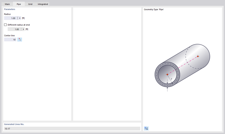
If the pipe cross-section is conical, activate the 'Different radius at end' check box and enter the corresponding value.

Spline with minimum curvature

With this geometry type, you can create a curved surface using control nodes that lie on or outside the surface. For example, terrain surfaces can be modeled in this way.

Define the 'coordinate system' of the reference plane and enter the 'sample coordinates in the coordinate system'. These points represent the control nodes of the spline surface. Then define the 'boundary lines of the reference plane' or select the lines graphically via the button.

Thickness with material

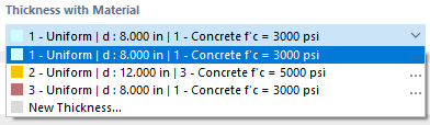
Select the suitable type from the list of existing thicknesses or define a new thickness (see chapter Thicknesses).

Material of thickness

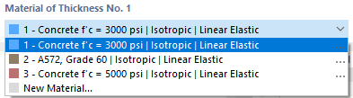
The material of the thickness defined in the section above is preset. If necessary, you can select a different material from the list of already created materials or define a new one (see chapter Materials). This material is then assigned to the thickness type.

Hinges

A hinge can be used to control the transfer of internal forces along a line of the surface (see chapter Line hinges. After checking the check box, you can define the hinge type in the 'Hinges' tab.

Support

If the surface is elastically supported, you can select or redefine the surface support in the 'Support' tab (see chapter Surface supports).

Release

To decouple the model at the surface, you can select or redefine a surface release in the 'Release' tab (see chapter Surface releases).

Eccentricity

An eccentricity allows a height offset of the entire surface to be modeled (see chapter Surface eccentricities). You can define the offset type in the 'Eccentricity' tab.

Load distribution factor

For a surface of the load transfer type, it is possible to define distribution factors for the load-bearing objects. If you check the check box, you can assign these factors individually in a new tab.

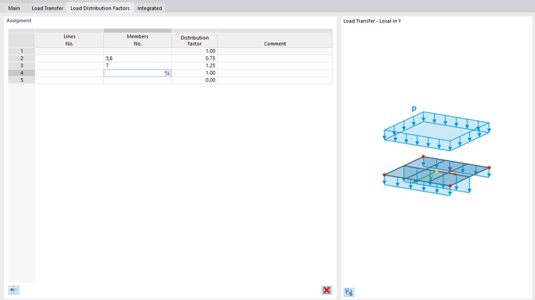
The loaded objects of the load transfer surface are preset in one row. Each object is assigned the factor 1.00, so that all objects contribute equally to the load transfer. If you want a specific distribution, click in the next free row and select the line or member. Then assign the appropriate 'distribution factor'.

Mesh refinement

The mesh size of the FE mesh can be adapted to the geometry of the surface (see chapter Surface mesh refinements). It is thus independent of the general mesh settings. In the 'Mesh refinement' tab, you can select or redefine the surface mesh refinement.

Specific axes

Each surface has a local coordinate system. As a rule, it is aligned parallel to the global axes. However, the coordinate system can also be defined by the user – separately for input and output.

Input axes

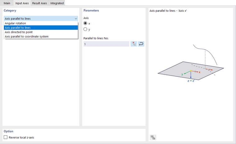
The orientation of the input axes is important, for example, for orthotropy and foundation properties or for the effect of a surface load.

The list in the 'Category' section offers various options for adjusting the axis position:

• Angular rotation: rotation of the xy surface axes about the z-axis by the angle α
• Axis parallel to lines: orientation of the x or y axis along a line
• Axis directed to point: orientation of the x or y axis to the intersection of a line with the surface
• Axis parallel to coordinate system: orientation of the axes to a user-defined coordinate system

You can determine the reference objects graphically via the button.

The 'Reverse local axis z' check box allows the z and y axes to be oriented in opposite directions.

Result axes

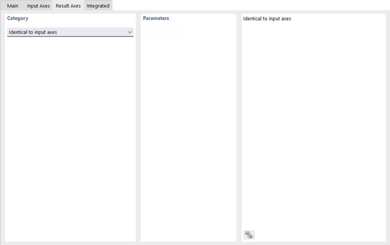
Currently, the orientation of the result axes is only possible 'identical to the input axes'.

Grid for results

Each surface is overlaid with a grid that is used for the result output in the tables. It enables an output independent of the FE mesh in regular, adjustable result points.

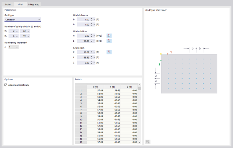
By default, a Cartesian surface grid with a uniform spacing of the grid points of 0.5 m in both directions is preset. If necessary, you can adjust the 'grid spacings' in the x-direction (b) and in the y-direction (h) here, perform a 'grid rotation', or change the 'grid origin'. For circular surfaces, the 'polar' grid type offers an alternative for the numerical result output.

If the 'Automatically adjust' check box is checked in the 'Options' section, the grid points are adapted to the new geometry when the surface is changed.

In the 'Points' section, you can check the coordinates of the generated grid points. Changes in the table are not possible.

Integrated objects

RFEM usually automatically detects all objects that lie in the surface but were not used for the surface definition.

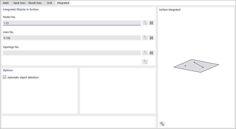
The numbers of the nodes, lines, and openings belonging to the surface are given in the 'Integrated objects in surface' section.

If an object is not detected, you should integrate it manually: Deactivate the automatic object detection. The input fields in the 'Integrated objects in surface' section are now accessible. Add the missing object number or use the button to determine the object graphically.

Activate load transfer

The check box makes it possible to distribute the load on the surface – regardless of its stiffness type – using a load transfer surface. This means that the surface acts in the model through its stiffness. The distribution of the load to the adjacent objects, on the other hand, is controlled by the parameters that you can define in the Load transfer tab. This function is primarily relevant for surfaces of the beam panel thickness type.

Deactivate for calculation

The check box offers the possibility not to take the surface into account in the calculation, for example to simulate construction stages or to examine a modeling variant. In this case, the stiffness, boundary conditions, and loads of the surface are not applied.

Information | Analytical

This section is displayed as soon as you have defined the boundary lines of the surface. It provides an overview of important properties of the surface such as surface area, solid, and mass, as well as the position of the surface centroid and the orientation of the surface. Openings are taken into account accordingly.