


In the Settings and Options tab, you can adjust the value of the acceleration of gravity, the geometric tolerances of the objects, and the alignment of the axes, as well as make settings for automatically connecting objects and for cost determination.
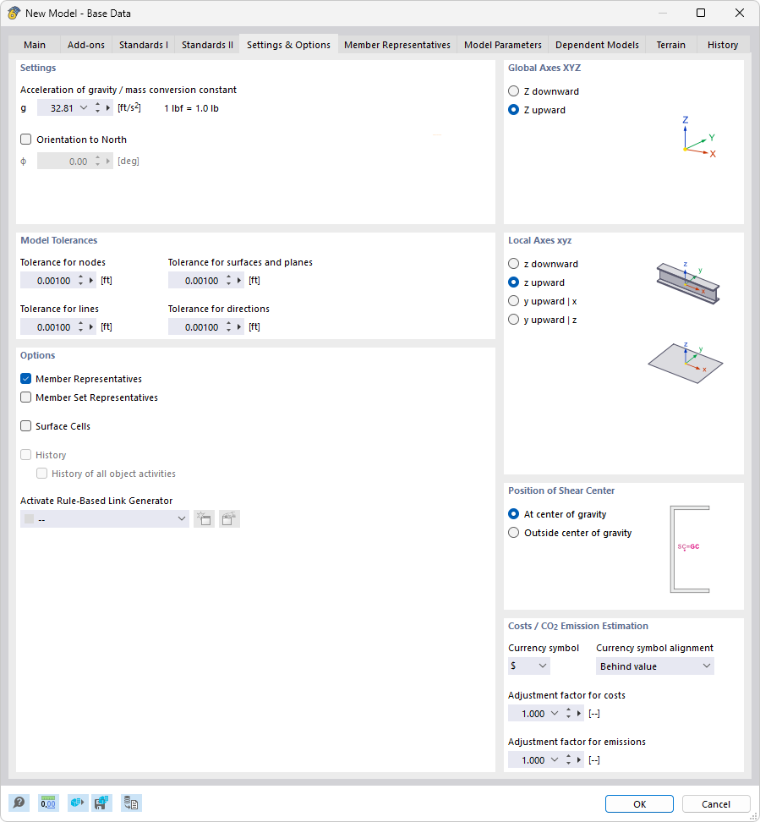
Settings
In this section, you can check the value of the 'gravitational acceleration' g. It is used for determining the self-weight of the members and surfaces, the conversion of masses ("mass conversion constant"), and for dynamic analyses. The approximate value of 10.00 m/s2 is preset by default and can be adjusted if necessary.
The 'alignment to the north' describes the position of the model relative to the main cardinal direction. A north orientation of 0° is preset by default, which corresponds to a northward alignment along the global X-axis. If you want to change the alignment of the model, activate the check box and enter the angle Φ.
Model Tolerances
When modeling or importing data from a CAD program, slight geometric differences may occur in the model objects. RFEM automatically cleans up these inconsistencies if certain distances are fallen below. For example, nodes lying very close to each other are merged, lines or members located outside of planes are integrated into surfaces, or minimally inclined lines and members are classified as vertical.
The preset tolerances are suitable for most models. For small model dimensions, it may be necessary to adjust the tolerances accordingly.
Options
The options in this section control whether so-called "representatives" for members and member sets or "surface cells" are used in the model.
If the check boxes for 'member representatives' and 'member set representatives' are activated, the additional tabs Member Representatives and Member Set Representatives are available in the dialog box. If the 'surface cells' check box is selected, the program automatically detects closed subareas of surfaces. This object type is described in the chapter Surface Cells.
The 'Enable rule-based coupling generator' list offers the possibility to use a generator for coupling unconnected model objects. This function is described in the chapter Rule-Based Coupling Generator. Using the
 button, you can create a new generator; using the
 button, you can edit the entry selected in the list.
Global Axes XYZ
This section controls the alignment of the global Z-axis. In CAD applications, the Z-axis usually points upwards, in structural analysis programs downwards. This does not matter for the calculation.
If Z is directed upwards, the factor -1.0 in Z is automatically applied for the 'active self-weight' function in the load case (see chapter load cases ).
Local Axes xyz
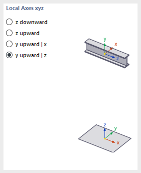
The designations of the member axes are regulated differently in the standards. Here you can define how the member main axes z or y and the surface axis z are aligned in order to adapt the local axis systems to the regional conventions.
The position of the local member and surface axes is illustrated in the graphics of this section.
Position of Shear Center
Using the two selection fields, you can control the influence of the shear center in the calculation with six degrees of freedom. In the predecessor versions, the position of the shear center was implicitly assumed to be 'at the center of gravity', so that no intended torsion could arise due to the cross-section geometry. The 'outside the center of gravity' option now offers the possibility to realistically represent the torsional behavior of asymmetric cross-sections.
Cost / CO2 Emission Estimation
The determination of the costs and CO2 emissions of a model is based on the member, surface, and solid elements of the model. For this purpose, a method is used that is also applied in practice for calculating the total costs of a building. The model is divided into units such as basement ceiling, exterior wall, or downstand beam. For these units, specific unit costs are developed that cover all costs to be recorded (price per surface, price per length, price per weight). The masses of the individual units (weight, volume, surface) are then multiplied by the associated unit costs. In this way, the partial costs for each unit are obtained. The sum of all partial costs gives the total costs of the model. The estimation of CO2 emissions is based on the same approach.
Define the currency symbol of the costs. You can then define the costs per unit for the materials and objects.
The adjustment factors allow you to globally scale the costs and CO2 emissions of the model. This can be helpful for cost adjustments in the course of the project.