Back to Online Manuals

10342x

000076

Dipl.-Ing. Frank Faulstich

2023-12-14

Select Manual

Overview

Graphical User Interface and Settings

Dlubal Center

Model Base Data

Structure

Imperfections

Load Cases and Combinations

Load Wizards

Loads

Result Objects

Costs and Emissions

Calculation

Results

Guide Objects

Digital Twins

Program Functions

Result Evaluation

Printout Reports

Drawing Sheets

Nonlinear Material Behavior

Material Models

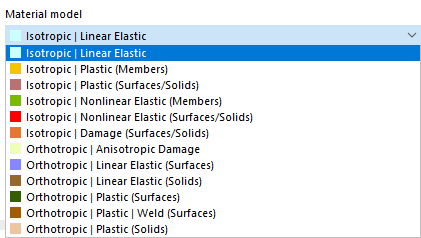
If the Nonlinear Material Behavior analysis add-on (requires a license) is activated in the Model Base Data, further options are available in the list of material models in addition to the Isotropic | Linear Elastic and | Linear Elastic material models.

Material Models for Nonlinear Material Behavior Add-on

Calculation Method

If you use a nonlinear material model, an iterative calculation is always performed. Depending on the material model, a different relation between the stresses and strains is defined.

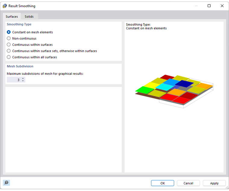
The stiffness of the finite elements is repeatedly adjusted in the course of the iterations until the stress-strain relation is complied with. The adjustment is always carried out for an entire surface or solid element. The Constant on mesh elements smoothing type should, therefore, always be used when evaluating stresses.

Result Smoothing

Plastic and Non-Elastic Material Models

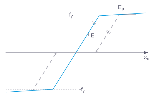
Some material models in RFEM are labeled as "Plastic", others as "Nonlinear Elastic". If a structural component with a nonlinear elastic material is relieved of loads again, the strain decreases along the same path. When the load is completely removed, no strain remains.

Stress-Strain Diagram for Nonlinear Elastic

When a component is relieved of loads with a plastic material model, a strain remains after complete unloading.

Stress-Strain Diagram for Plastic

Loading and unloading can be simulated using the Construction Stages Analysis add-on.

Tip

Further information about nonlinear elastic material models can be found in the technical article Yield Laws in Isotropic Nonlinear Elastic Material Model.

Surface Internal Forces

The internal forces in plates with nonlinear material result from the numerical integration of the stresses over the plate thickness. To define the integration method for the thickness, select the Specify integration method option in the "Edit Thickness" dialog box. The following integration methods are available:

Gauss-Lobatto quadrature
Simpson's rule
Trapezoidal rule

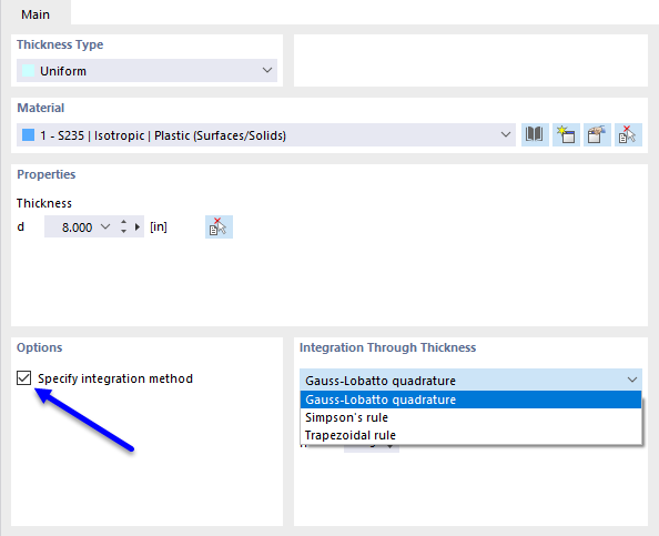
Defining Integration Method for Surface Thickness

You can also specify the "Number of integration points" from 3 to 99 via the plate thickness.

Tip

Theoretical background on the individual integration methods can be found in the Multilayer Surfaces manual.

Isotropic | Plastic (Members)

If you select Isotropic | Plastic (Members) from the "Material model" drop-down list, the tab for entering the nonlinear material parameters is activated.

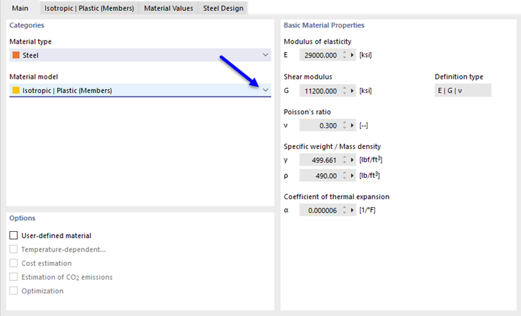
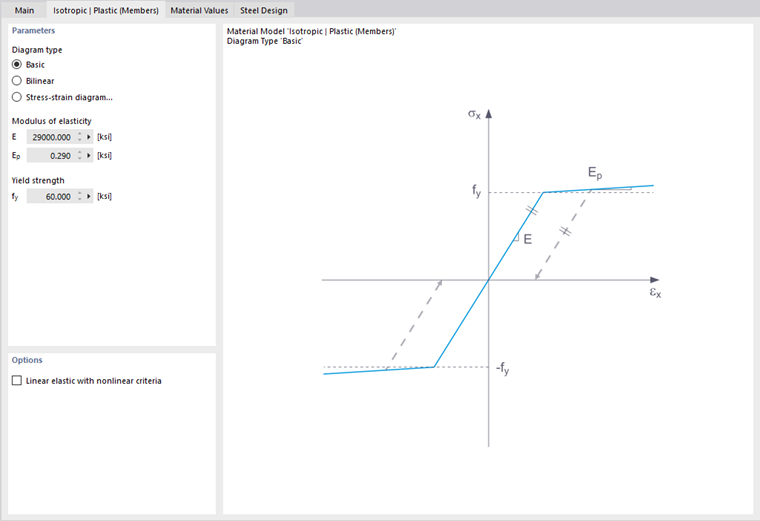
Activating Nonlinear Material Model

Defining Nonlinear Material Parameters

In this tab, you define the stress-strain diagram. The following options are available:

Basic
Bilinear
Diagram

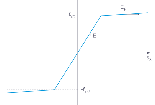
If you select Basic, RFEM uses a bilinear material model. The values from the material library are used for the modulus of elasticity E and the yield strength f_y. For numerical reasons, the diagram branch is not exactly horizontal, but has a small slope E_p.

If you want to change the values for the yield strength and the modulus of elasticity, activate the User-defined material check box in the "Main" tab.

Activating User-Defined Material

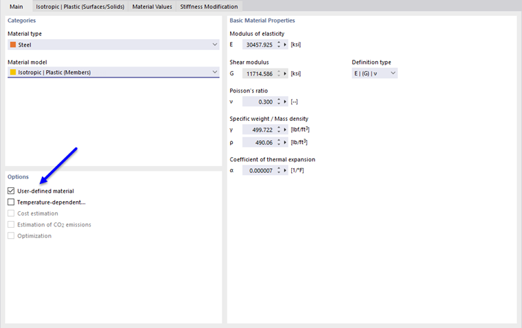
For a bilinear definition, you can also enter a value for E_p.

More complex relations between stress and strain can be defined by means of the Stress-strain diagram. If you select this option, the "Stress-Strain Diagram" tab is displayed.

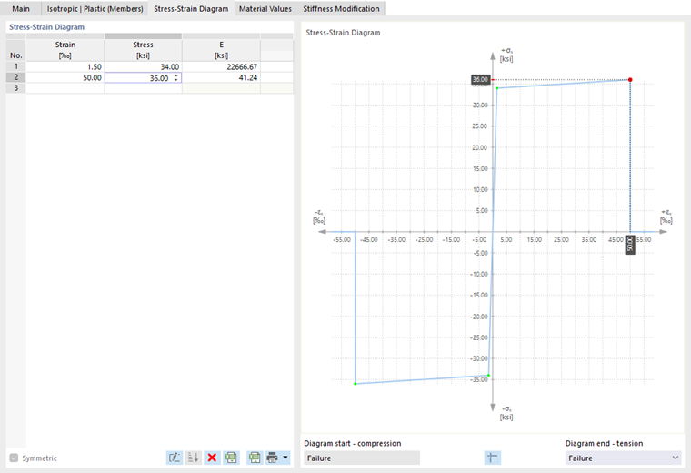
Entering a user-defined stress-strain diagram

Entering User-Defined Stress-Strain Diagram

Define a point for the stress-strain relation in each table row. You can select how the diagram continues after the last definition point in the "Diagram end" list below the diagram:

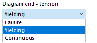
Distribution after the last definition point

Distribution After Last Definition Point

In the case of "Failure", stress after the last definition point jumps back to zero (for example, when material tears). "Yielding" means that stress remains constant when strain increases. "Continuous" means that the graph continues with the slope of the last section.

Info

In this material model, the stress-strain diagram refers to the longitudinal stress σ_x. Different yield strengths for tension and compression cannot be taken into account with this material model.

Isotropic | Plastic (Surfaces/Solids)

If you select Isotropic | Plastic (Surfaces/Solids) from the "Material model" drop-down list, the tab for entering the nonlinear material parameters is activated.

Selecting Plastic Material Model

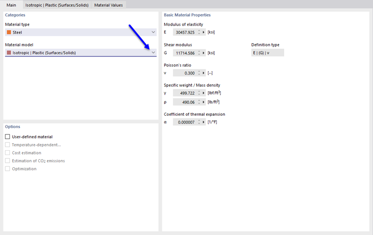
First, select the "Stress failure hypothesis". The following hypotheses are available for selection:

von Mises (von Mises yield criterion)
Tresca (Tresca yield criterion)
Drucker-Prager
Mohr-Coulomb

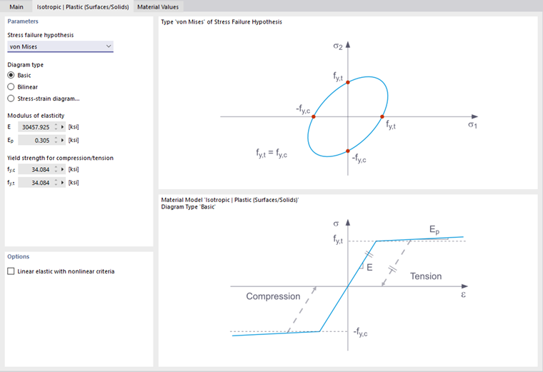
Defining Stress Failure Hypothesis

If you select von Mises, the following stresses are used in the stress-strain diagram:

Surfaces

σ_{v} = \sqrt{σ_{x}^{2} + σ_{y}^{2} - σ_{x} σ_{y} + 3 (τ_{xy}^{2})}

Equivalent Stress from Basic Stresses According to von Mises

Solids

σ_{v, Mises} = \sqrt{σ_{x}^{2} + σ_{y}^{2} + σ_{z}^{2} - σ_{x} σ_{y} - σ_{x} σ_{z} - σ_{y} σ_{z} + 3 (τ_{xy}^{2} + τ_{xz}^{2} + τ_{yz}^{2})}

Equivalent Stress σ_v,Mises from Basic Stresses

σ_{v, Mises} = \sqrt{\frac{1}{2} [(σ_{1} - σ_{2})^{2} + (σ_{1} - σ_{3})^{2} + (σ_{2} - σ_{3})^{2}]}

Equivalent Stress σ_v,Mises from Principal Stresses

According to the Tresca hypothesis, these stresses are used:

Surfaces

σ_{v} = \sqrt{{(σ_{x} - σ_{y})}^{2} + 4 {τ_{xy}}^{2}}

Equivalent Stress According to Tresca

Solids

σ_{v, Tresca} = max (|σ_{1} - σ_{2}|; |σ_{2} - σ_{3}|; |σ_{3} - σ_{1}|)

Equivalent Stress σ_v,Tresca

According to the Drucker-Prager hypothesis, the following stress is used for surfaces and solids:

σ_{v} = \frac{m - 1}{2} (σ_{1} + σ_{2} + σ_{3}) + \frac{m + 1}{2} \sqrt{\frac{1}{2} [{(σ_{1} - σ_{2})}^{2} + {(σ_{2} - σ_{3})}^{2} + {(σ_{3} - σ_{1})}^{2}]}

m = \frac{σ_{c}}{σ_{t}}

σ_c	Limit stress for compression
σ_t	Limit stress for tension

Yield Criterion According to Drucker-Prager

According to the Mohr-Coulomb hypothesis, the following stress is used for surfaces and solids:

σ_{v} = \frac{m + 1}{2} \max \{|σ_{1} - σ_{2}| + K (σ_{1} + σ_{2}), |σ_{2} - σ_{3}| + K (σ_{2} + σ_{3}), |σ_{3} - σ_{1}| + K (σ_{3} + σ_{1})\}

K = \frac{m - 1}{m + 1}

m = \frac{σ_{c}}{σ_{t}}

Mohr – Coulomb

Isotropic | Nonlinear Elastic (Members)

The functionality largely corresponds to that of the Plastic (Members) material model. But in contrast to it, no plastic strain remains after the load is removed.

Isotropic | Nonlinear Elastic (Surfaces/Solids)

The functionality largely corresponds to that of the Plastic (Surfaces/Solids) material model. But in contrast to it, no plastic strain remains after the load is removed.

Isotropic | Damage (Surfaces/Solids)

In contrast to other material models, the stress-strain diagram for this material model is not antimetric to the origin. This material model can, therefore, be used to model the behavior of steel fiber-reinforced concrete, for example. Detailed information on modeling steel fiber-reinforced concrete can be found in this technical article on the Material Properties of Steel-Fiber-Reinforced Concrete.

Material Model "Isotropic | Damage"

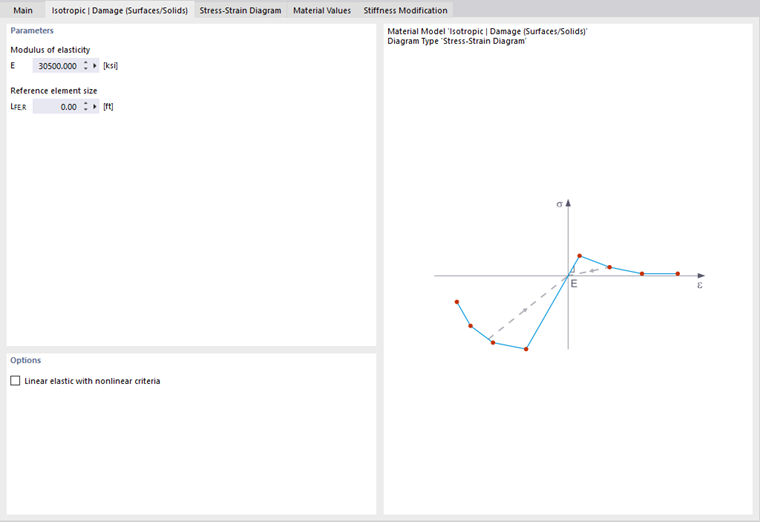
The isotropic stiffness is reduced with a scalar damage parameter. This damage parameter is determined from the stress curve defined in the Diagram. This does not take the direction of the principal stresses into account; rather, the damage occurs in the direction of the equivalent strain, which also covers the third direction perpendicular to the plane. The tension and compression areas of the stress tensor are treated separately. Different damage parameters apply in each case.

The "Reference element size" controls how the strain in the crack area is scaled to the length of the element. With the default value zero, no scaling is performed. Thus, the material behavior of the steel fiber-reinforced concrete is modeled realistically.

Tip

Theoretical background on the "Isotropic Damage" material model can be found in the technical article Nonlinear Material Model Damage.

Orthotropic | Anisotropic Damage

Timber materials have direction-dependent (anisotropic) properties. The principal anisotropic directions are along the grain, radial, and tangential. In the Orthotropic | Anisotropic Damage tab, you can define the nonlinear properties.

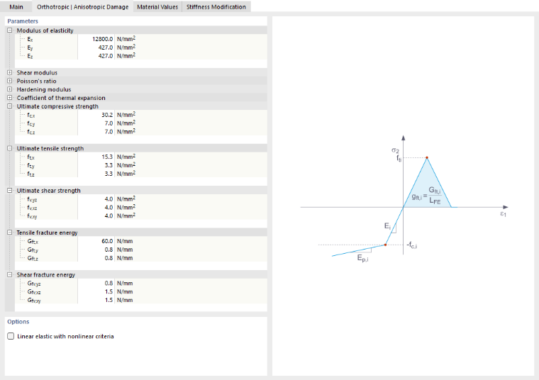
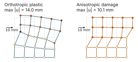
Material Model "Orthotropic | Anisotropic Damage"

This material model implements Sandhaas’s damage model [2] with eight failure criteria for timber. Timber behaves as quasi-brittle under tension and shear and as ductile under compression. It fails in planes determined by the grain direction. The model according to [2] describes eight separate failure criteria (one for each quadrant of the stress space), which are controlled by nine stiffness reduction factors.

The local x-axis has a parallel distribution relative to the grain, the y-axis has a radial distribution, and the z-axis has a tangential distribution. Each criterion is a stress function F that reaches a value of 1 at the onset of damage. Four of these are simple maximum stress criteria. The four criteria for transverse tension and shear are elliptical: Fracturing in a planar environment can be triggered by tension perpendicular to it, by shear along the plane, or
by any combination thereof.

Specify the ultimate strength of the material, as well as the tensile fracture energy and shear fracture energy for each direction.

Info

Unlike the Orthotropic | Plastic material model, the forces are not redistributed, but decoupled by the failure of the fiber plane. This allows you to model the splitting behavior of timber. The deformations are generally smaller.

Deformations for the Orthotropic | Plastic (left) and Orthotropic | Anisotropic damage (right) material model

Deformations for Material Model Orthotropic | Plastic (Left) and Orthotropic | Anisotropic Damage (Right)

Orthotropic | Plastic (Surfaces) / Plastic (Solids)

The material model according to "Tsai-Wu" unifies plastic with orthotropic properties. This allows for special modeling of materials with anisotropic characteristics, such as fiber-reinforced plastics or timber.

If the material is plastified, the stresses remain constant. A redistribution takes place depending on the stiffnesses that are present in the individual directions.

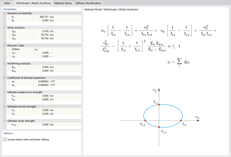
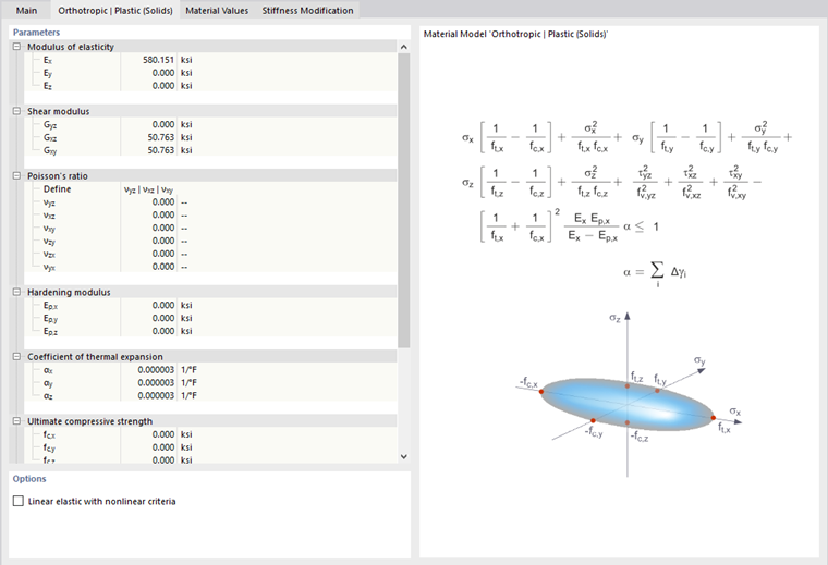
Material Model "Orthotropic | Plastic (Surfaces)"

Material Model "Orthotropic | Plastic (Solid)"

The elastic area corresponds to the material model Linear Elastic (Solids). The following yielding condition according to Tsai-Wu applies to the plastic zone:

Surfaces

σ_{x} [\frac{1}{f_{t, x}} - \frac{1}{f_{c, x}}] + \frac{{σ_{x}}^{2}}{f_{t, x} f_{c, x}} +

σ_{y} [\frac{1}{f_{t, y}} - \frac{1}{f_{c, y}}] + \frac{{σ_{y}}^{2}}{f_{t, y} f_{c, y}} +

\frac{{τ_{xy}}^{2}}{{f_{v, xy}}^{2}} - {[\frac{1}{f_{t, x}} + \frac{1}{f_{c, x}}]}^{2} \frac{E_{x} E_{p, x}}{E_{x} - E_{p, x}} α \leq 1

α = \sum_{i} ∆ γ_{i}

Tsai-Wu, State of Plane Stress

Solids

σ_{x} [\frac{1}{f_{t, x}} - \frac{1}{f_{c, x}}] + \frac{{σ_{x}}^{2}}{f_{t, x} f_{c, x}} +

σ_{y} [\frac{1}{f_{t, y}} - \frac{1}{f_{c, y}}] + \frac{{σ_{y}}^{2}}{f_{t, y} f_{c, y}} +

σ_{z} [\frac{1}{f_{t, z}} - \frac{1}{f_{c, z}}] + \frac{{σ_{z}}^{2}}{f_{t, z} f_{c, z}} +

\frac{{τ_{yz}}^{2}}{{f_{v, yz}}^{2}} + \frac{{τ_{xz}}^{2}}{{f_{v, xz}}^{2}} + \frac{{τ_{xy}}^{2}}{{f_{v, xy}}^{2}} -

{[\frac{1}{f_{t, x}} + \frac{1}{f_{c, x}}]}^{2} \frac{E_{x} E_{p, x}}{E_{x} - E_{p, x}} α \leq 1

α = \sum_{i} ∆ γ_{i}

Tsai-Wu, Spatial State of Stress

All strengths are to be defined as positive.

The yield condition can be imagined as an elliptical surface in the six-dimensional stress space. If one of the three stress components is applied as a constant value, the surface can be projected onto a three-dimensional stress space.

If the value for f_y(σ) according to the Tsai-Wu, plane stress state equation is less than 1, the stresses are in the elastic range. The plastic range is reached as soon as f_y(σ) = 1. Values greater than 1 are not allowed. The model behavior is ideal-plastic, which means there is no stiffening.

Orthotropic | Plastic | Weld (Surfaces)

This material model is used in analyses with the Steel Joints add-on to represent the behavior of welds in accordance with standards. Only stresses that correspond to the stress components σ_⊥, τ_⊥, and τ_|| of the weld occur in the equivalent surface. In the other stress directions, the stiffness of the equivalent surface approaches zero.

Material Model "Orthotropic | Plastic | Weld (Surfaces)"

In the "Orthotropic | Plastic | Weld (Surfaces)" tab, you can define the parameters for taking plastic strain hardening for welds into account, such as the limit values f_ekv and f_x for the stress analysis according to the "Directional Method" as per EN 1993-1-8 [1] for welds, modified by a plastic component (see also the technical article Design of Fillet Welds).

Concrete

The nonlinear material models Anisotropic | Damage and Isotropic | Damage (Surfaces/Solids) are available for the "Concrete" material type.

Material Models for Concrete

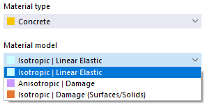
The material models are described in the chapter Anisotropic | Damage of the Concrete Design manual or above in the Isotropic Damage section.

Masonry

If the Masonry Design add-on (requires a license) is activated in the Model Base Data, the nonlinear material models "Isotropic | Masonry | Plastic (Surfaces)" and "Orthotropic | Masonry | Plastic (Surfaces)" are available for selection for the "Masonry" material type.

Material Models for Masonry

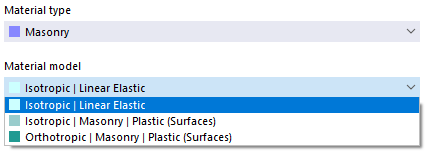
Both material models are described in the chapter Materials of the Masonry Design manual.

Fabric

The material library contains two rows for the material type “fabric”:

Glass-PTFE: Glass fabric coated with polytetrafluoroethylene (PTFE)
PES-PVC: Polyester fabric coated with polyvinyl chloride (PVC)

Info

The “Foil” material type is intended for foils, such as ETFE.

For fabric materials the nonlinear material model Orthotropic | Fabric | Nonlinear Elastic (Surfaces) is available in addition to the orthotropic linear material model.

Material Models for Fabric

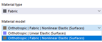
This material model allows for a realistic modeling of the orthotropic behavior of prestressed fabric membranes, whose stiffnesses in the warp and weft directions differ. It describes the fabric using a representative solid element (RVE) of its microstructure. By considering the fabric geometry, the model simnulates the corresponding transverse strain effect for all force states in the membrane. Since the load-dependent stiffness behavior of the fabric is also taken into account, it is possible to perform an accurate analysis of membrane structures.

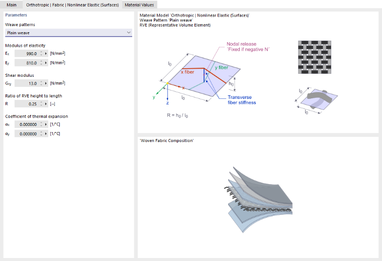
Material Model "Orthotropic | Fabric | Nonlinear Elastic (Surfaces)"

The properties of fabrics are determined in biaxial tests, which result in the moduli of elasticity E_x and E_y, as well as the shear modulus G_xy. However, the coupling between the warp and weft directions arises from the geometry of the fibers: under load, the crimp (ondulation) of the fibers changes in both directions. This effect is referred to in English as “crimp interchange.” The material model therefore derives the material response from a unit cell of the fabric structure. This unit cell also includes its own geometric nonlinearity. Poisson's ratios are not used in this model. The coupling between the two directions is achieved via the parameter R of the unit cell.

As with all nonlinear elastic material models, the strain reverts to its original state along the same path during load relief. The calculation is performed iteratively.

Material Model "Orthotropic | Fabric | Nonlinear Elastic (Surfaces)"

Select the fabric’s manufacturing type from the “Weave patterns” list. Two options are available:

Plain weave
Panama weave

Specify the modulus of elasticity in the x- and y-direction. Since the shear moduli G_yz and G_xz are always zero for fabrics, only the G_xy input box for the Poisson's ratio in the fabric plane is provided. This shear modulus may also be zero.

The parameter R describes the ratio of the height to the length of the representative solid element (RVE). This value must be between 0 and 1.

R = \frac{h_{0}}{l_{0}}

h₀	Height of the unit cell perpendicular to the membrane plane
l₀	Length of the unit cell

Parameter R of Unit Cell

For materials from the library, R = 0.25 is the default setting and, like the other properties, cannot be changed. For a user-defined material, you can adjust R.

If necessary, adjust the thermal expansion coefficients of the fabric: α_x in the warp direction and α_y in the weft direction. They may also be zero.

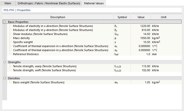
In the “Material Values” tab, the properties of a fabric are specified according to industry standards in the membrane industry. The x-direction corresponds to the warp direction, and the y-direction corresponds to the weft direction.

Tab "Material Values"

Fabric Thickness

The thickness of a membrane is very small and can hardly be determined with certainty. In the membrane industry, stiffness and strength are therefore related to the width, for example, in kN/m. RFEM follows this convention and converts the values to stress quantities using the reference thickness t_ref.

E_{x} = \frac{E_{x, MV}}{t_{ref}} E_{y} = \frac{E_{y, MV}}{t_{ref}} G_{x y} = \frac{G_{x y, MV}}{t_{ref}}

E_x,MV / E_y,MV / G_xy,MV	Stiffness values in the “Material Properties” tab
t_ref	Reference thickness

Conversion of Stiffnesses

These values appear in the Material Values tab. When you assign a fabric to a thickness, RFEM uses the material’s reference thickness t_ref as the thickness d.

The membrane stiffness E_x·t_ref corresponds to the width-related value in the library. Deformations and membrane forces, such as n_x and n_y in kN/m, therefore do not depend on the numerical value of the reference thickness, as long as all properties are related to the same reference thickness. Stresses, on the other hand, are related to the reference thickness.

Info

The strengths f_x,k,23 and f_y,k,23, as well as the weight per unit area m_s, have no influence on the calculation. The strengths are available for design checks.

If you change the reference thickness for a user-defined material in the “Material Values” tab, this affects the material properties in the material model tab. Therefore, first define the reference thickness and then the stiffnesses.

Notes on Form-Finding and Design

The form-finding process is independent of the material. The fabric properties have no influence on the resulting shape. They only affect the subsequent calculation under load. The fundamentals are described in the chapter Form-Finding Process of the Form-Finding manual.

Tip

Membrane structures behave in a highly nonlinear manner. If the calculation does not converge, first check the model: All membrane surfaces and cables should have a form-finding load, and all membrane edges should be supported by cables or line supports.

A constant orthotropic prestress is physically unachievable for doubly curved surfaces. If you combine orthotropic prestressing with a very large number of form-finding iterations using the standard method, tangential sliding motions in the membrane plane, unstable convergence, and large deformations in the plane may occur. This behavior is independent of the material model. Use the preset number of iterations or select the projection method.

References

European Committee for Standardization. (2010). Eurocode 3: Design of Steel Structures – Part 1-8: Design of Joints. Brussels: CEN.
Sandhaas, C. (2012). Mechanical Behaviour of Timber Joints with Slotted-in Steel Plates. Dissertation, TU Delft.

Parent Chapter